Methodology for Surfaces Analysis and Classification
Andrej Cupar
1,*, Vojko Pogačar
1, Zoran Stjepanović
21University of Maribor, Faculty of Mechanical Engineering Maribor, Department of Structures and Design, Laboratory for Design,
Smetanova 17, 2000, Maribor, Slovenia
2University of Maribor, Faculty of Mechanical Engineering Maribor, Department of Textile Materials and Design, Smetanova 17, 2000,
Maribor, Slovenia
*Corresponding Author: [email protected]
Copyright © 2014 Horizon Research Publishing All rights reserved.
Abstract
We present analysis methodology for differenttypes of geometry. This is needed for classification methodology of surfaces. We have proposed several classes and ways to place surfaces in proper classes, according to their characteristic curves. Several state-of-the-art cases were analysed with Grasshopper (GH) procedure. Classes are explained and some shapes are tested. Classification is necessary for further design improvement and analysis of existing geometry.
Keywords
Surfaces classification, Design, Analysis,3D scan, Curvature graph
1. Introduction and Objectives
There have been some classifications and surface evaluations made, but none is universal and complete. We have been researching the possibilities of our GH procedure. There are many fields where such analytic approach can be used; it can be aesthetic, quality measurement or any other purpose.
A well-designed product can be brought to marked earlier. Already existing objects can be analysed and evaluated. Or aesthetics can be proofed.
We are operating with geometry that mathematically describes real-world objects. Therefore approximation and simplification is needed for successful work. In design, mainly fair curves are used: a curve is fair if its curvature plot is continuous and consist of only a few monotone pieces [1]. Methods for analysing curve’s aesthetic impression have already been developed. Those curves are parts of logarithmic graphs. Researchers observed graph curvature in dependence of path – K(s) and K-vector in logarithmic curvature histogram (LCH) [2]. Researchers Kanaya et al. [3], used this method to determine an objects' impression. They found out that Japanese observed objects have convergent impression and European objects divergent impression. Harada defined aesthetic curve as a curve whose LCH is a straight line. On the basis of LCHs he proposed five
general classes for aesthetic curves: minus, zero, plus, plus-minus and minus-plus [2]. Kanaya uses LCH on characteristic curves on cars side views and also on 3D scans. There have been used series of curves to analyse impression of analysed surface [3]. Other authors have also observed and analysed spatial aesthetic curve segments [4]. They created graphs K(s) and LCHs of those curves.
Some leading researchers participated in the project FIORES II [5–7]. They proposed several terms for styling properties and features in Computer Aided Industrial Design (CAID). By means of questions and observation of communication between stylists and engineers they built a list of terms that describes styling properties and features; these are:
Radius/Blending
Convex/Concave
Tension
Straight/Flat
Hollow
Lead in
Soft/Sharp
S-Shaped
Crown
Hard/Crude
Acceleration [5–7].
All researchers do not use all terms. Anyway, they agree this list is not complete or perfect. Some of the terms are similar; or rather the same characteristic planar curve can be described with several terms [6].
2. Methods
2.1. Grasshopper
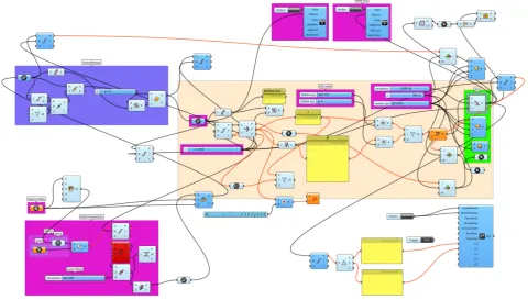
Figure 1. Sample of quite complex GH’s procedure.
Procedures are created by dragging components on a canvas. Outputs of these components are then connected to the inputs of subsequent components.
Grasshopper is mainly used to build generative algorithms. Many of Grasshopper’s components create 3D geometry. Procedures may also contain other types of algorithms, including numeric, textual, audio-visual or haptic applications [9].
2.2. Grasshopper Procedure
GH’s procedure computes points, which represent graphs of curvature – K(s). This procedure can become very complex, Figure 1. We can import any geometry and connect it into the procedure to get an appropriate graph. Both, geometry and graph, can be then exported in many computer formats in Rhinoceros (RH) for further use. We will take these mathematical tools as they are and will not research how they get the results.
2.3. Curvature Graph
We will use K(s) graphs and not LCH’s because of disorder in LCH representation for complex geometry of 3D scanned objects.
Several classifications of specific geometries were already done by some other researchers. Poldermann[10], who seems to work especially with sheet metal design, and does not attach our work. Classification of fully freeform surfaces was made by Cheutet[11]. This classification took in view progress of logarithmic histogram of curvature which was
used on aesthetic curves [12]. A new classification and parametric representation of freeform features was presented by He[13].
Planar curve is given by Cartesian parametric equations: 𝑥𝑥 = 𝑥𝑥(𝑡𝑡) and 𝑦𝑦 = 𝑦𝑦(𝑡𝑡) (1) Then the curvature K, sometimes named the “first curvature”, is defined by:
𝐾𝐾 =𝑑𝑑∅𝑑𝑑𝑑𝑑 = 𝑑𝑑∅𝑑𝑑𝑡𝑡 𝑑𝑑𝑑𝑑 𝑑𝑑𝑡𝑡
= 𝑑𝑑∅𝑑𝑑𝑡𝑡 ��𝑑𝑑𝑥𝑥
𝑑𝑑𝑡𝑡� 2
+�𝑑𝑑𝑦𝑦𝑑𝑑𝑡𝑡�2 = 𝑑𝑑∅ 𝑑𝑑𝑡𝑡
�𝑥𝑥′2+𝑦𝑦′2 (2) Where ∅ is the tangential angle and s is the arc length. With some improvements we can write:
𝐾𝐾 =(𝑥𝑥′𝑥𝑥′𝑦𝑦2+𝑦𝑦′′′−𝑦𝑦′𝑦𝑦′′2)3/2 (3) For two dimensional curve in the form 𝑦𝑦 = 𝑓𝑓(𝑥𝑥), the equation of curvature becomes:
𝐾𝐾 = 𝑑𝑑2𝑦𝑦𝑑𝑑𝑥𝑥2 �1+�𝑑𝑑𝑦𝑦𝑑𝑑𝑥𝑥�2�
3/2 (4)
With considered circles that are tangent to the curve at given point:
𝑥𝑥 = 𝜌𝜌 cos 𝑡𝑡 (5) 𝑦𝑦 = 𝜌𝜌 sin 𝑡𝑡 (6) The definition of curvature of surface curve equals:
[image:2.595.66.547.79.352.2]2.4. Lasses
According to results of the researches provided by the project FIORES II, we propose the framework of the following shape classes:
Convex/Concave
Accelerated/Decelerated
Solid/Slim
Technical/Organic
Sharp/Soft
Combined
All the classes consist of two opposite extremes. In the future we are going to simplify the names or choose only one.
The Convex/Concave class describes shapes which are not flat or straight but have some changes in curvature and do not show any direction. This means that the shape is symmetric in the prescribed limits.
The Accelerated/Decelerated class also contains shapes
with curvature changes and shows direction, which means, an accelerated shape is not symmetric.
The Solid/Slim class uses length to width ratio to assign this class to shape.
The Technical/Organic class integrates shapes with very dynamic curvature progress for organic on one side or quite static curvature progress on other, for technical surface.
Sharp/Soft means intensity of curvature change. Sharp shows very concentrate change and soft names surfaces that have distributed curvature change.
The Combined class combines two or more properties of other classes.
2.5 Analysis types and methods
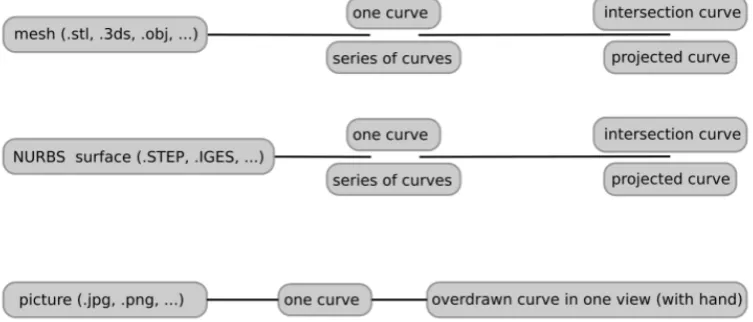
Different types of geometry can be analysed in different ways (Figure 2). But always is a single curve or series of curves needed for further analysis.
Figure 2. Different types of geometry can be analysed in different ways.
[image:3.595.118.495.310.471.2] [image:3.595.127.488.513.631.2]2.5.1 Mesh
Mesh is very common computer file format for storing geometry. 3D scans are usually represented as mesh. If mesh is clean, without any bulges or holes; we can use it as it is for further analysis. Otherwise, we have to clean and repair that mesh (Figure 4).
Figure 4. Mesh that has to be cleaned and repaired.
2.5.2. NURBS Surface
BREP (boundary representation) geometry can be reverse engineered geometry out of a 3D scan, or a newly designed surface. We usually do not have problems with newly designed surfaces. On the other hand, the reverse engineered surfaces may contain irregularities that were scanned from real object. Hereinafter, a cleaned surface can be reverse engineered.
2.5.3. Overdrawn Curve
An overdrawn curve should be planar so we can operate with pictures or 3D geometry. A curve can be as accurate as needed. We can overdraw it by hand or automatically. A new curve shall be of proper degree and shall describe the main shape of the object. Irregularities from scanned mesh should be correctly smoothed. An overdrawn curve shows main characteristic of the object and we get it from side, front, rear or top of the object. Rotated planes of views were rarely needed.
We get the B-spline, which can be written as:
𝐶𝐶(𝑡𝑡) = ∑
𝑛𝑛𝑖𝑖=0𝑃𝑃
𝑖𝑖𝑁𝑁
𝑖𝑖,𝑝𝑝(𝑡𝑡)
(8)Where
𝑃𝑃
0, … 𝑃𝑃
𝑛𝑛 are control points and𝑁𝑁
𝑖𝑖,𝑝𝑝 is basis function [14, 17]. This curve is analysed in the GH procedure later on.2.5.4. Intersection
Two meshes were imported in the procedure for mesh intersection. On the intersection we get polyline, interpolated in curve, which gets input for the rest of the procedure. This part of the procedure is useful if we have mesh objects like a 3D scan. The shape resulting graphs do not depend on the position of the 3D object. Therefore, interaction can be
defined for two surfaces. We simply add a proper mesh for the intersection. This can be a simple plane or any other geometry. It is necessary to adjust a polyline with the reduce tool. This is later divided with points. Through these points, a curve is interpolated and finally fitted. Parameters can be adjusted, and we get best results with fitted curve from 0 to 0.1.
2.5.5. Projected Curve
[image:4.595.59.299.158.320.2]A curve can be projected on a mesh or on any BREP (boundary representation) geometry. By this means, we get a curve for further analysis that is shown on (Figure 5), where is line projected on ellipsoid. Then we get ellipse, where K(s) graph can be calculated, shown on the right side.
Figure 5. Line is projected on ellipsoid.
3. Results with Discussion
3.1 Cultural Heritage
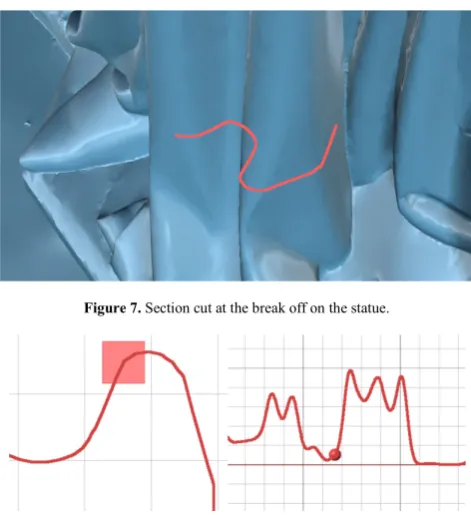
[image:4.595.314.550.251.339.2]Analysis of the main altar of Mantled Virgin Mary on Ptujska Gora, Slovenia [18], shows irregularity at Virgin Mary’s feet, Figure 6. Red circle marks the place, where the irregularity appears.
Figure 6. 3D scanned altar of Mantled Virgin Mary on Ptujska Gora, Slovenia.
[image:4.595.316.551.488.655.2]Figure 7. Section cut at the break off on the statue.
Figure 8. K(s) graph on the top and intersection curve at the bottom.
3.2. Symmetry
Symmetry can be confirmed with our procedure. For perfect symmetry K(s) graph is also symmetric. K(s) can be exported as points in an spreadsheet document. Y coordinates at symmetric points are then equal.
Figure 9. Symmetry of a curve at the top and its K(s) graph at the bottom.
Figure 9 shows perfect symmetry for B-spline. That confirms procedure’s correctness. Hereinafter, roof section cut of 3D modelled car was analysed, Figure 10. Although the car was modelled from scratch in Maya, where it was mirrored in modelling process, our procedure shows imperfect symmetry. This probably came from errors in saving files.
Figure 10. Symmetry of the roof on the car and corresponding K(s) on the right.
Figure 11. Symmetry of 3D scanned Michelangelo’s David statue, actually his copy.
David’s statue as an aesthetic ideal of human body shows almost perfect symmetry (Figure 11). Then again, an average human face in Figure 12 shows some more deviation from perfect symmetry that cannot be seen on a section cut curve. K(s) graph drastically increases changes that are not visible directly on a section cut curve. There are three waves. The middle one represents nose and other two the cheekbones on each side.
Figure 12. Symmetry of 3D scanned human face.
3.3. Class evaluation
[image:5.595.319.547.74.189.2]Proposed classes can include surfaces and curves[19]. Convex/Concave surface has typical K(s) graph procedure convex curve. An accelerated surface has falling K(s), a decelerated one has a growing graph. An organic surface has very irregular and distorted K(s) graph. A technical surface K(s) has horizontal lines and GH procedure usually produces errors because of straight lines that have infinite curvature. Solid/Slim describes surfaces that have ratio of their bounding box within predicted limits. Sharp/Soft indicates connection of surfaces and graphs that are sharp or soft as well.
[image:5.595.323.541.327.445.2] [image:5.595.80.275.441.526.2] [image:5.595.321.544.639.721.2] [image:5.595.69.295.641.733.2]Accelerate curves show properties of a curve with energy that falls from the left to the right side, Figure 13. At the upper left side is the most accelerated curve and every curve has less acceleration in direction downwards [5]. It is opposite with decelerated curves on the right – energy grows from the left to the right: they are mirrored over vertical axis.
Figure 14. Convex curves at the top and at the bottom mirrored concave curves and their K(s) graphs.
Convex and concave curves have identic K(s) graphs for same curved curves Figure 14. Therefore, we have to add the sign in name to uniquely mark each one.
[image:6.595.98.254.158.318.2]Curves with more convexity or concavity have lower extremes at K(s) graphs. With increasing of convexity or concavity we get sharp curve, described hereinafter.
Figure 15. Organic curve at the top and technical curve at the bottom and their K(s) graphs.
Organic curve can be in future joined with Convex/Concave class, because it consists of small parts of convex and concave curves, (Figure 15).
Figure 16: Sharp curve at the top and at the bottom soft curve and their K(s) graphs.
3.3.1. Computer mouse analysis
Figure 17. Longitudinal section cut on a computer mouse.
Figure 18. On the right is K(s) of longitudinal section cut on computer mouse.
According to our classes, the longitudinal section cut on a computer mouse in Figure 17 belongs in decelerated class, shown in Figure 18 on the right.
Figure 19. Left-sided section cut on a computer mouse.
Figure 20. K(s) of left-sided section cut on a computer mouse (on the right).
The side section cut on a computer mouse in (Figure 19) belongs to the Concave class, (Figure 20 on the right). But for a non-ambiguous claim we need to know the side of material, while the same section curve would mean Convex class because K(s) is the same for both.
[image:6.595.310.554.395.548.2] [image:6.595.62.300.442.564.2] [image:6.595.382.494.578.643.2] [image:6.595.64.293.643.733.2]mathematical background. The K(s) graph is independent from orientation in space, but the size does affect it. We have implemented part of procedure that normalizes geometry. This means all curves are the same size and can be compared. Therefore is K(s) graph in our GH procedure also size independent.
Surface irregularities that cannot be seen with naked eye can be detected on any 3D scanned object, not only on those, belonging to cultural heritage. Anyway, the procedure needs improvements and testing.
In order to determine the proper class, we also need to know the side of material, to know if a surface middle goes in or out of the object, where K(s) does not detect that. That should be applied to Convex/Concave and Accelerated/Decelerated classes. Proposed classed come in pairs that describe two opposite properties. Number of those pairs is limited, similar to the colour theory. There are three major opposition axes. Two are chromatic and one achromatic. All other colours between them in colour space are mixtures [20]. It is the same with our classes. There is limited number of major classes, all others are derivates.
As expected, the results of GH procedure are not always perfect. But main progress of K(s) graph can be compared to reference graphs in chapter Class evaluation.
4. Conclusions
Great potential and extension of our methodology can be found in intelligent support systems, where it can be implemented. [21-23]
The number of classes has to be revised and probably be reduced. Parameters optimization of the procedure and some other improvements has to be done in future research.
Classification and evaluation of surfaces will be our future work. The connection to colour theory, sound theory and all sorts of electromagnetic waves is evident. Hopefully, a widely recognized shape classification space will exist very soon, similar to the well-known colour space.
REFERENCES
[1] G. Farin, Curves and Surfaces for CAGD: A Practical Guide. Morgan Kaufmann Publishers, USA 2002.
[2] T. Harada, F. Yoshimoto, and M. Moriyama, An Aesthetic Curve in the Field of Industrial Design, Proceedings of the IEEE Symposium on Visual Languages, 38, 1999.
[3] I. Kanaya, Y. Nakano, and K. Sato, Simulated Designer’s Eyes – Classification of Aesthetic Surfaces, Proc. Int’l Conf. Virtual Systems and Multimedia. 289–296, 2003.
[4] N. Yoshida and T. Saito, Compound-Rhythm Log-Aesthetic Curves, Computer Aided Design & Applications Vol. 6, No. 1, 1–10, 2009.
[5] F. Giannini, M. Monti, and G. Podehl, Styling properties and
features in computer aided industrial design, Computer Aided Design & Applications, Vol. 1, No. 1–4, 321–330, 2004.
[6] F. Giannini, M. Monti, and G. Podehl, Aesthetic-driven tools for industrial design, Journal of Engineering Design, Vol. 17, No. 3, 193–215, 2006.
[7] G. Podehl, Terms and Measures for Styling Properties, 7th International Design Conference – Design 2002, 879–886, 2002.
[8] Scott Davidson, Grasshopper, Online Available from: http://www.grasshopper3d.com
[9] Wikipedia, Grasshopper3d, Online Available from: http://en.wikipedia.org/wiki/Grasshopper_3d
[10] B. Poldermann, Surface Design Based on Parametrized Surface features, Proceedings of the International Symposium on Tools and Methods for Concurrent Engineering, Budapest Technical University Press, Budapest, 1995.
[11] V. Cheutet, C.E. Catalano, J.P. Pernot, B. Falcidieno, F. Giannini, and J.C. Leon, 3D Sketching for Aesthetic Design Using Fully Free-form Deformation Deatures, Computers & Graphics, vol. 29, no. 6, 916–930, 2005.
[12] N. Yoshida and T. Saito, Interactive Aesthetic Curve Segments, The Visual Computer, Vol. 22, No. 9–11. 896–905, 2006.
[13] K. He, Z. Chen, and L. Zhao, A New Method for Classification and Parametric Representation of Freeform Surface Feature, International Journal of Advanced Manufacturing Technology, Vol. 57, No. 1–4, 271–283, 2011.
[14] G. Farin, J. Hoschek, and M.-S. Kim, Handbook of computer aided geometric design. Amsterdam, Elsevier, 2002.
[15] Wolfram Math World, curvature. Online Available from: http://mathworld.wolfram.com/Curvature.html.
[16] L.A. Piegl Tiller, Wayne, The NURBS Book. Springer–Verlag New York, 1997.
[17] WolframMathWorld. Online Available from:
http://mathworld.wolfram.com/B-Spline.html.
[18] Slotraveler.com, Ptujska Gora. Online Available from: http://www.ptujskagora.eu/slhtml.
[19] A. Cupar, V. Pogacar, Z. Stjepanovic, Methodology for Analysing Digitised Geometry, DAAAM International Scientific Book 2013, DAAAM International, Vienna, Austria, 2013.
[20] V. Pogacar, System of colour dominance based on semantical logic of natural cycles, Proceedings of the 11th Congress of the International Colour Association, 2009. [21] J. Kaljun, B. Dolšak, Ergonomic Design Knowledge built in
the Intelligent Decision Support System, International Journal of Industrial Ergonomics, Vol. 42, No. 1, 162-171, 2012.
[22] B. Dolšak, M. Novak, Intelligent Decision Support for Structural Design Analysis, Advanced Engineering Informatics, Vol. 25, No. 2, 330-340, 2011.