Li n e a r di s c ri mi n a n t a n a ly si s : a
d e t a il e d t u t o ri al
G a b er, T, T h a r w a t , A, I b r a h i m , A a n d H a s s a n i e n , AE
h t t p :// dx. d oi.o r g / 1 0 . 3 2 3 3 /AIC-1 7 0 7 2 9
T i t l e
Li n e a r di s c ri mi n a n t a n a ly si s : a d e t ail e d t u t o ri al
A u t h o r s
G a b er, T, T h a r w a t , A, I b r a h i m , A a n d H a s s a n i e n , AE
Typ e
Ar ticl e
U RL
T hi s v e r si o n is a v ail a bl e a t :
h t t p :// u sir. s alfo r d . a c . u k /i d/ e p ri n t/ 5 2 0 7 4 /
P u b l i s h e d D a t e
2 0 1 7
U S IR is a d i gi t al c oll e c ti o n of t h e r e s e a r c h o u t p u t of t h e U n iv e r si ty of S alfo r d .
W h e r e c o p y ri g h t p e r m i t s , f ull t e x t m a t e r i al h el d i n t h e r e p o si t o r y is m a d e
f r e ely a v ail a bl e o nli n e a n d c a n b e r e a d , d o w nl o a d e d a n d c o pi e d fo r n o
n-c o m m e r n-ci al p r iv a t e s t u d y o r r e s e a r n-c h p u r p o s e s . Pl e a s e n-c h e n-c k t h e m a n u s n-c ri p t
fo r a n y f u r t h e r c o p y ri g h t r e s t r i c ti o n s .
1
Linear Discriminant Analysis: A Detailed
Tutorial
Alaa Tharwat
∗Department of Computer Science and Engineering, Frankfurt University of Applied Sciences, Frankfurt am Main, Germany
Faculty of Engineering, Suez Canal University, Egypt E-mail: [email protected]
Tarek Gaber
∗Faculty of Computers and Informatics, Suez Canal University, Egypt
E-mail: [email protected]
Abdelhameed Ibrahim
∗Faculty of Engineering, Mansoura University, Egypt Email: [email protected]
Aboul Ella Hassanien
∗Faculty of Computers and Information, Cairo University, Egypt
E-mail: [email protected]
∗Scientific Research Group in Egypt, (SRGE), http://www.egyptscience.net
Linear Discriminant Analysis (LDA) is a very common technique for dimensionality reduction problems as a pre-processing step for machine learning and pattern classifica-tion applicaclassifica-tions. At the same time, it is usually used as a black box, but (sometimes) not well understood. The aim of this paper is to build a solid intuition for what is LDA, and how LDA works, thus enabling readers of all levels be able to get a better understanding of the LDA and to know how to apply this technique in different applications. The paper first gave the basic definitions and steps of how LDA technique works supported with visual explanations of these steps. Moreover, the two methods of computing the LDA space, i.e.
class-dependent and class-independent methods, were ex-plained in details. Then, in a step-by-step approach, two nu-merical examples are demonstrated to show how the LDA space can be calculated in case of the class-dependent and class-independent methods. Furthermore, two of the most common LDA problems (i.e.Small Sample Size(SSS) and non-linearity problems) were highlighted and illustrated, and state-of-the-art solutions to these problems were investigated
and explained. Finally, a number of experiments was con-ducted with different datasets to (1) investigate the effect of the eigenvectors that used in the LDA space on the robust-ness of the extracted feature for the classification accuracy, and (2) to show when theSSSproblem occurs and how it can be addressed.
Keywords: Dimensionality reduction, PCA, LDA, Kernel Functions, Class-Dependent LDA, Class-Independent LDA, SSS (Small Sample Size) problem,, eigenvectors artificial in-telligence
1. Introduction
Dimensionality reduction techniques are important in many applications related to machine learning [15], data mining [6,33], Bioinformatics [47], biometric [61] and information retrieval [73]. The main goal of the mensionality reduction techniques is to reduce the di-mensions by removing the redundant and dependent features by transforming the features from a higher di-mensional space that may lead to a curse of dimension-ality problem, to a space with lower dimensions. There are two major approaches of the dimensionality reduc-tion techniques, namely, unsupervised and supervised approaches. In the unsupervised approach, there is no need for labeling classes of the data. While in the su-pervised approach, the dimensionality reduction tech-niques take the class labels into consideration [32,15]. There are many unsupervised dimensionality reduc-tion techniques such as Independent Component Anal-ysis (ICA) [31,28] and Non-negative Matrix Factor-ization (NMF) [14], but the most famous technique of the unsupervised approach is the Principal Component Analysis (PCA) [71,4,67,62]. This type of data reduc-tion is suitable for many applicareduc-tions such as visualiza-tion [40,2], and noise removal [70]. On the other hand, the supervised approach has many techniques such as Mixture Discriminant Analysis (MDA) [25] and Neu-ral Networks (NN) [27], but the most famous technique of this approach is the Linear Discriminant Analysis (LDA) [50]. This category of dimensionality reduction
AI Communications
techniques are used in biometrics [36,12], Bioinfor-matics [77], and chemistry [11].
The LDA technique is developed to transform the features into a lower dimensional space, which max-imizes the ratio of the between-class variance to the within-class variance, thereby guaranteeing maximum class separability [76,43]. There are two types of LDA technique to deal with classes: class-dependent and
class-independent. In the class-dependent LDA, one separate lower dimensional space is calculated for each class to project its data on it whereas, in the class-independent LDA, each class will be considered as a separate class against the other classes [1,74]. In this type, there is just one lower dimensional space for all classes to project their data on it.
Although the LDA technique is considered the most well-used data reduction techniques, it suffers from a number of problems. In the first problem, LDA fails to find the lower dimensional space if the dimensions are much higher than the number of samples in the data matrix. Thus, the within-class matrix becomes singu-lar, which is known as thesmall sample problem(SSS). There are different approaches that proposed to solve this problem. The first approach is to remove the null space of within-class matrix as reported in [79,56]. The second approach used an intermediate subspace (e.g. PCA) to convert a within-class matrix to a full-rank matrix; thus, it can be inverted [35,4]. The third ap-proach, a well-known solution, is to use the regulariza-tion method to solve a singular linear systems [38,57]. In the second problem, the linearity problem, if differ-ent classes are non-linearly separable, the LDA can-not discriminate between these classes. One solution to this problem is to use the kernel functions as reported in [50].
The brief tutorials on the two LDA types are re-ported in [1]. However, the authors did not show the LDA algorithm in details using numerical tutorials, vi-sualized examples, nor giving insight investigation of experimental results. Moreover, in [57], an overview of the SSS for the LDA technique was presented in-cluding the theoretical background of the SSS prob-lem. Moreover, different variants of LDA technique were used to solve the SSS problem such as Di-rect LDA (DLDA) [22,83], regularized LDA (RLDA) [18,37,38,80], PCA+LDA [42], Null LDA (NLDA) [10,82], and kernel DLDA (KDLDA) [36]. In addition, the authors presented different applications that used the LDA-SSS techniques such as face recognition and cancer classification. Furthermore, they conducted dif-ferent experiments using three well-known face
recog-nition datasets to compare between different variants of the LDA technique. Nonetheless, in [57], there is no detailed explanation of how (with numerical exam-ples) to calculate the within and between class vari-ances to construct the LDA space. In addition, the steps of constructing the LDA space are not supported with well-explained graphs helping for well understanding of the LDA underlying mechanism. In addition, the non-linearity problem was not highlighted.
This paper gives a detailed tutorial about the LDA technique, and it is divided into five sections. Section 2 gives an overview about the definition of the main idea of the LDA and its background. This section begins by explaining how to calculate, with visual explanations, the between-class variance, within-class variance, and how to construct the LDA space. The algorithms of cal-culating the LDA space and projecting the data onto this space to reduce its dimension are then introduced. Section 3 illustrates numerical examples to show how to calculate the LDA space and how to select the most robust eigenvectors to build the LDA space. While Sec-tion 4 explains the most two common problems of the LDA technique and a number of state-of-the-art meth-ods to solve (or approximately solve) these problems. Different applications that used LDA technique are in-troduced in Section 5. In Section 6, different packages for the LDA and its variants were presented. In Section 7, two experiments are conducted to show (1) the influ-ence of the number of the selected eigenvectors on the robustness and dimension of the LDA space, (2) how theSSSproblem occurs and highlights the well-known methods to solve this problem. Finally, concluding re-marks will be given in Section 8.
2. LDA Technique
2.1. Definition of LDA
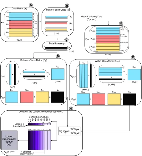
within-class variance. This section will explain these three steps in detail, and then the full description of the LDA algorithm will be given. Figures (1 and 2) are used to visualize the steps of the LDA technique.
2.2. Calculating the Between-Class Variance (SB)
The between-class variance of theithclass (S Bi)
rep-resents the distance between the mean of theith class (µi) and the total mean (µ). LDA technique searches
for a lower-dimensional space, which is used to max-imize the between-class variance, or simply maxi-mize the separation distance between classes. To ex-plain how the class variance or the between-class matrix (SB) can be calculated, the following
as-sumptions are made. Given the original data matrix
X={x1,x2, . . . ,xN}, where xi represents theith
sam-ple, pattern, or observation and N is the total num-ber of samples. Each sample is represented byM fea-tures (xi∈
R
M). In other words, each sample isrepre-sented as a point inM-dimensional space. Assume the data matrix is partitioned intoc=3 classes as follows,
X= [ω1,ω2,ω3]as shown in Fig. (1, step (A)). Each
class has five samples (i.e.n1=n2=n3=5), whereni
represents the number of samples of theith class. The total number of samples (N) is calculated as follows,
N=∑3i=1ni.
To calculate the between-class variance (SB), the
separation distance between different classes which is denoted by(mi−m)will be calculated as follows:
(mi−m)2= (WTµi−WTµ)2=WT(µi−µ)(µi−µ)TW
(1) wheremirepresents the projection of the mean of the ith class and it is calculated as follows, mi =WTµi,
where m is the projection of the total mean of all classes and it is calculated as follows, m=WTµ,W
represents the transformation matrix of LDA1,µi(1× M)represents the mean of theith class and it is com-puted as in Equation (2), andµ(1×M)is the total mean of all classes and it can be computed as in Equation (3) [83,36]. Figure (1) shows the mean of each class and the total mean in step (BandC), respectively.
µj=
1
njxi
∑
∈ωjxi (2)
1The transformation matrix (W) will be explained in Sect. 2.4
µ= 1
N N
∑
i=1 xi=
c
∑
i=1 ni
Nµi (3)
wherecrepresents the total number of classes (in our examplec=3).
The term (µi−µ)(µi−µ)T in Equation (1)
repre-sents the separation distance between the mean of the
ithclass (µi) and the total mean (µ), or simply it repre-sents the between-class variance of theith class (S
Bi).
SubstituteSBi into Equation (1) as follows:
(mi−m)2=WTSBiW (4)
The total between-class variance is calculated as fol-lows, (SB=∑ci=1niSBi). Figure (1, step (D)) shows first
how the between-class matrix of the first class (SB1) is calculated and then how the total between-class matrix (SB) is then calculated by adding all the between-class
matrices of all classes.
2.3. Calculating the Within-Class Variance (SW)
The within-class variance of theith class (SWi)
rep-resents the difference between the mean and the sam-ples of that class. LDA technique searches for a lower-dimensional space, which is used to minimize the dif-ference between the projected mean (mi) and the
pro-jected samples of each class (WTxi), or simply min-imizes the class variance [83,36]. The within-class variance of each within-class (SWj) is calculated as in
Equation (5).
∑
xi∈ωj,j=1,...,c
(WTxi−mj)2
=
∑
xi∈ωj,j=1,...,c
(WTxi j−WTµj)2
=
∑
xi∈ωj,j=1,...,c
WT(xi j−µj)2W
=
∑
xi∈ωj,j=1,...,c
WT(xi j−µj)(xi j−µj)TW
=
∑
xi∈ωj,j=1,...,c
WTSWjW
(5) From Equation (5), the within-class variance for each class can be calculated as follows,SWj=d
T j∗dj=
∑ni=j1(xi j−µj)(xi j−µj)T, where xi jrepresents the ith
WTSBWff WTSwW argfmax=
μ1 μ
μ1
μ
dMx1E
d1xME
SB1=
Between-ClassfMatrixfdSBE
dn1xME
Sw1=
-μ1
ω1
-ω1 μ1
Within-ClassfMatrixfdSWE
D=
dNxME
ω1-μ1
ω2-μ2
ω3-μ3
x1-μ1 x2-μ1 xn1-μ1 xdn1L1E-μ2 xdn1Ln2E-μ2
xN-μ3 d1xME
μ1
μ2
μ3
MeanfoffeachfClassfdμiE
-μ
d1xME TotalfMeanfdμE
Vk∈RMxK
dMxn1E
X =
SB1
SB1 SB2 SB3
SB=
SB
L L =
X
--
-
=SW1
SW1 SW2 SW3
SW=
SW
L L =
v1v2 vk vM
λ1λ2 λM
SortedfEigenvalues
λk
Largestfkf Eigenvalues
kfSelected Eigenvectors
Lowerf Dimensionalf
Space dVkE
dMxME dMxME
B
C
D F
G
E
ConstructfthefLowerfDimensionalfSpacefdVkE
ω1
ω2
ω3
X=
x1 x2
xn1
dNxME
xn1L1 xn1L2
xn1Ln2
xN
DatafMatrixfdXE
A
Mean-CenteringfDataf
dDi=ωi-μiE
[image:5.595.61.515.119.618.2]W
Fig. 1. Visualized steps to calculate a lower dimensional subspace of the LDA technique.
F)), anddj is the centering data of the jth class, i.e. dj=ωj−µj={xi}
nj
i=1−µj. Moreover, step (F) in the
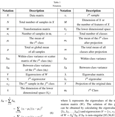
Table 1 Notation.
Notation Description Notation Description
X Data matrix xi ithsample
N Total number of samples inX M Dimension ofXor
the number of features ofX
W Transformation matrix Vk The lower dimensional space
ni Number of samples inωi c Total number of classes
µi
The mean of
theithclass mi
The mean of theithclass after projection
µ Total or global mean
of all samples m
The total mean of all classes after projection
SWi
Within-class variance or scatter matrix of theithclass (ωi)
SW Within-class variance
SBi
Between-class variance of theithclass (ωi)
SB Between-class variance
V Eigenvectors ofW λ Eigenvalue matrix
Vi itheigenvector λi itheigenvalue
xi j Theithsample in the jthclass Y Projection of the original data
k The dimension of the lower
dimensional space (Vk)
ωi ithClass
SW = 3
∑
i=1 SWi
=
∑
xi∈ω1
(xi−µ1)(xi−µ1)T
+
∑
xi∈ω2
(xi−µ2)(xi−µ2)T
+
∑
xi∈ω3
(xi−µ3)(xi−µ3)T
(6)
2.4. Constructing the Lower Dimensional Space
After calculating the between-class variance (SB)
and within-class variance (SW), the transformation
ma-trix (W) of the LDA technique can be calculated as in Equation (7), which is called Fisher’s criterion. This formula can be reformulated as in Equation (8).
arg max W
WTS BW WTS
WW
(7)
SWW =λSBW (8)
where λ represents the eigenvalues of the
transfor-mation matrix (W). The solution of this problem can be obtained by calculating the eigenvalues (λ= {λ1,λ2, . . . ,λM}) and eigenvectors (V={v1,v2, . . . ,vM})
ofW=SW−1SB, ifSW is non-singular [83,36,81]. The eigenvalues are scalar values, while the eigen-vectors are non-zero eigen-vectors, which satisfies the Equa-tion (8) and provides us with the informaEqua-tion about the LDA space. The eigenvectors represent the directions of the new space, and the corresponding eigenvalues represent the scaling factor, length, or the magnitude of the eigenvectors [59,34]. Thus, each eigenvector rep-resents one axis of the LDA space, and the associated eigenvalue represents the robustness of this eigenvec-tor. The robustness of the eigenvector reflects its ability to discriminate between different classes, i.e. increase the between-class variance, and decreases the within-class variance of each within-class; hence meets the LDA goal. Thus, the eigenvectors with thekhighest eigen-values are used to construct a lower dimensional space (Vk), while the other eigenvectors ({vk+1,vk+2,vM})
Projection
Y
∈
R
NxkData1After1Projection
k
V
k∈R
MxKLower1
Dimensional1
Space
(V
k)
ω1
ω2
ω3
X=
x1
x2
xn1
(NxM)
xn1+1
xn1+2
xn1+n2
xN
Data1Matrix1(X)
ω1
ω2
ω3
y1
y2
yn1
yn1+1
yn1+2
yn1+n2
yN
[image:7.595.69.509.106.290.2]Y=XV
kFig. 2. Projection of the original samples (i.e. data matrix) on the lower dimensional space of LDA (Vk).
Figure (2) shows the lower dimensional space of the LDA technique, which is calculated as in Fig. (1, step (G)). As shown, the dimension of the original data matrix (X ∈
R
N×M) is reduced by projecting it ontothe lower dimensional space of LDA (Vk∈
R
M×k) asdenoted in Equation (9) [81]. The dimension of the data after projection isk; hence,M−kfeatures are ig-nored or deleted from each sample. Thus, each sample (xi) which was represented as a point aM-dimensional
space will be represented in ak-dimensional space by projecting it onto the lower dimensional space (Vk) as
follows,yi=xiVk.
Y=XVk (9)
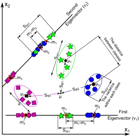
Figure (3) shows a comparison between two lower-dimensional sub-spaces. In this figure, the original data which consists of three classes as in our example are plotted. Each class has five samples, and all sam-ples are represented by two features only (xi ∈
R
2)to be visualized. Thus, each sample is represented as a point in two-dimensional space. The transforma-tion matrix (W(2×2)) is calculated using the steps in Sect. 2.2, 2.3, and 2.4. The eigenvalues (λ1andλ2)
and eigenvectors (i.e. sub-spaces) (V={v1,v2}) ofW
are then calculated. Thus, there are two eigenvectors or sub-spaces. A comparison between the two lower-dimensional sub-spaces shows the following notices:
– First, the separation distance between different classes when the data are projected on the first eigenvector (v1) is much greater than when the
data are projected on the second eigenvector (v2).
As shown in the figure, the three classes are effi-ciently discriminated when the data are projected onv1. Moreover, the distance between the means
μ1
μ2
μ3 μ S
W2 SW1
S
W3
SB3
SB2 SB1
x1 x2
m2 m1
m3
The distance between cla
sses
The vara ince
within each class
First Eigenvector (v1) m1
m2
m3
m1-m2
m1-m 2
SW1 SW1
Second
Eigen vector (v
2)
Fig. 3. A visualized comparison between the two lower-dimensional sub-spaces which are calculated using three different classes.
of the first and second classes (m1−m2) when the
original data are projected onv1is much greater
than when the data are projected onv2, which
re-flects that the first eigenvector discriminates the three classes better than the second one.
– Second, the within-class variance when the data are projected onv1is much smaller than when it
projected onv2. For example,SW1 when the data are projected onv1is much smaller than when the
data are projected onv2. Thus, projecting the data
onv1minimizes the within-class variance much
[image:7.595.302.529.321.544.2]From these two notes, we conclude that the first eigen-vector meets the goal of the lower-dimensional space of the LDA technique than the second eigenvector; hence, it is selected to construct a lower-dimensional space.
2.5. Class-Dependent vs. Class-Independent Methods
The aim of the two methods of the LDA is to cal-culate the LDA space. In the class-dependent LDA, one separate lower dimensional space is calculated for each class as follows,Wi=SW−1iSB, whereWirepresents
the transformation matrix for the ithclass. Thus, eigen-values and eigenvectors are calculated for each trans-formation matrix separately. Hence, the samples of each class are projected on their corresponding eigen-vectors. On the other hand, in the class-independent method, one lower dimensional space is calculated for all classes. Thus, the transformation matrix is calcu-lated for all classes, and the samples of all classes are projected on the selected eigenvectors [1].
2.6. LDA Algorithm
In this section the detailed steps of the algorithms of the two LDA methods are presented. As shown in Algorithms (1 and 2), the first four steps in both al-gorithms are the same. Table (1) shows the notations which are used in the two algorithms.
2.7. Computational Complexity of LDA
In this section, the computational complexity for LDA is analyzed. The computational complexity for the first four steps, common in both class-dependent and class-independent methods, are computed as fol-lows. As illustrated in Algorithm (1), in step (2), to calculate the mean of theith class, there areniM
ad-ditions andMdivisions, i.e., in total, there are(NM+
cM) operations. In step (3), there are NM additions andM divisions, i.e., there are(NM+M)operations. The computational complexity of the fourth step is
c(M+M2+M2), whereM is forµi−µ,M2for(µi− µ)(µi−µ)T, and the lastM2is for the multiplication
betweenniand the matrix(µi−µ)(µi−µ)T. In the fifth
step, there areN(M+M2)operations, whereMis for
(xi j−µj)and M2 is for (xi j−µj)(xi j−µj)T. In the
sixth step, there areM3operations to calculateSW−1,M3
is for the multiplication betweenSW−1andSB, andM3
to calculate the eigenvalues and eigenvectors. Thus, in class-independent method, the computational
com-Algorithm 1.: Linear Discriminant Analysis (LDA):
Class-Independent
1: Given a set of N samples [xi]Ni=1, each of which
is represented as a row of lengthMas in Fig. (1, step(A)), andX(N×M)is given by,
X=
x(1,1) x(1,2) . . .x(1,M)
x(2,1) x(2,2) . . .x(2,M) ..
. ... ... ...
x(N,1)x(N,2). . .x(N,M)
(10)
2: Compute the mean of each classµi(1×M)as in Equation (2).
3: Compute the total mean of all dataµ(1×M)as in Equation (3).
4: Calculate between-class matrixSB(M×M)as
fol-lows:
SB= c
∑
i=1
ni(µi−µ)(µi−µ)T (11) 5: Compute within-class matrixSW(M×M), as
fol-lows:
SW = c
∑
j=1 nj
∑
i=1
(xi j−µj)(xi j−µj)T (12)
wherexi jrepresents theithsample in the jthclass. 6: From Equation (11 and 12), the matrix W that maximizing Fisher’s formula which is defined in Equation (7) is calculated as follows,W=SW−1SB.
The eigenvalues (λ) and eigenvectors (V) ofWare
then calculated.
7: Sorting eigenvectors in descending order accord-ing to their correspondaccord-ing eigenvalues. The firstk
eigenvectors are then used as a lower dimensional space (Vk).
8: Project all original samples (X) onto the lower di-mensional space of LDA as in Equation (9). plexity isO(NM2)ifN>M; otherwise, the complexity isO(M3).
In Algorithm (2), the number of operations to cal-culate the within-class variance for each class SWj in the sixth step is nj(M+M2), and to calculate SW, N(M+M2) operations are needed. Hence, calculat-ing the within-class variance for both LDA methods are the same. In the seventh step and eighth, there are M3 operations for the inverse, M3 for the multi-plication of S−W1
iSB, and M
3 for calculating
Algorithm 2.: Linear Discriminant Analysis (LDA): Class-Dependent
1: Given a set of N samples [xi]Ni=1, each of which
is represented as a row of lengthM as in Fig. (1, step(A)), andX(N×M)is given by,
X=
x(1,1) x(1,2) . . .x(1,M)
x(2,1) x(2,2) . . .x(2,M) ..
. ... ... ...
x(N,1)x(N,2). . .x(N,M)
(13)
2: Compute the mean of each classµi(1×M)as in Equation (2).
3: Compute the total mean of all dataµ(1×M)as in Equation (3).
4: Calculate between-class matrix SB(M×M) as in
Equation (11)
5: for allClassi,i=1,2, . . . ,cdo
6: Compute within-class matrix of each class
SWi(M×M), as follows:
SWj=
∑
xi∈ωj
(xi−µj)(xi−µj)T (14)
7: Construct a transformation matrix for each class (Wi) as follows:
Wi=SW−i1SB (15)
8: The eigenvalues (λi) and eigenvectors (Vi) of each transformation matrix (Wi) are then
calcu-lated, whereλi andVi represent the calculated eigenvalues and eigenvectors of theithclass, re-spectively.
9: Sorting the eigenvectors in descending order ac-cording to their corresponding eigenvalues. The firstkeigenvectors are then used to construct a lower dimensional space for each classVi
k. 10: Project the samples of each class (ωi) onto their
lower dimensional space (Vki), as follows:
Ωj=xiVkj, xi∈ωj (16)
where Ωj represents the projected samples of
the classωj. 11: end for
each class which increases the complexity of the class-dependent algorithm. Totally, the computational
com-plexity of the class-dependent algorithm isO(NM2)if
N>M; otherwise, the complexity isO(cM3). Hence,
the class-dependent method needs computations more than class-independent method.
In our case, we assumed that there are 40 classes and each class has ten samples. Each sample is rep-resented by 4096 features (M >N). Thus, the com-putational complexity of the class-independent method isO(M3) =40963, while the class-dependent method needsO(cM3) =40×40963.
3. Numerical Examples
In this section, two numerical examples will be pre-sented. The two numerical examples explain the steps to calculate the LDA space and how the LDA tech-nique is used to discriminate between only two differ-ent classes. In the first example, the lower-dimensional space is calculated using the class-independent method, while in the second example, the class-dependent method is used. Moreover, a comparison between the lower dimensional spaces of each method is presented. In all numerical examples, the numbers are rounded up to the nearest hundredths (i.e. only two digits after the decimal point are displayed).
The first four steps of both class-independent and class-dependent methods are common as illustrated in Algorithms (1 and 2). Thus, in this section, we show how these steps are calculated.
Given two different classes,ω1(5×2)andω2(6×2)
have (n1=5) and (n2=6) samples, respectively. Each
sample in both classes is represented by two features (i.e.M=2) as follows:
ω1=
1.00 2.00 2.00 3.00 3.00 3.00 4.00 5.00 5.00 5.00
andω2=
4.00 2.00 5.00 0.00 5.00 2.00 3.00 2.00 5.00 3.00 6.00 3.00
(17)
To calculate the lower dimensional space using LDA, first the mean of each classµjis calculated. The
total meanµ(1×2)is then calculated, which represents the mean of all means of all classes. The values of the mean of each class and the total mean are shown below,
µ1=3.00 3.60,µ2=4.67 2.00, and µ=5
11µ1 6 11µ2
=
The between-class variance of each class (SBi(2×
2)) and the total between-class variance (SB(2×2)are
calculated. The values of the between-class variance of the first class (SB1) is equal to,
SB1=n1(µ1−µ)T(µ1−µ) =5[−0.91 0.87]T[−0.91 0.87] =
4.13 −3.97
−3.97 3.81
(19) Similarly,SB2 is calculated as follows:
SB2=
3.44 −3.31
−3.31 3.17
(20) The total between-class variance is calculated a fol-lows:
SB=SB1+SB2 =
4.13 −3.97
−3.97 3.81
+
3.44 −3.31
−3.31 3.17
=
7.58 −7.27
−7.27 6.98
(21) To calculate the within-class matrix, first subtract the mean of each class from each sample in that class and this step is called mean-centering data and it is cal-culated as follows, di =ωi−µi, where di represents
centering data of the classωi. The values ofd1andd2
are as follows:
d1=
−2.00−1.60
−1.00−0.60 0.00 −0.60 1.00 1.40 2.00 1.40
andd2=
−0.67 0.00 0.33 −2.00 0.33 0.00
−1.67 0.00 0.33 1.00 1.33 1.00
(22) In the next two subsections, two different methods are used to calculate the LDA space.
3.1. Class-Independent Method
In this section, the LDA space is calculated using the class-independent method. This method represents the standard method of LDA as in Algorithm (1).
After centring the data, the within-class variance for each class (SWi(2×2)) is calculated as follows,
SWj =d
T
j ∗dj =∑ni=j1(xi j−µj)T(xi j−µj), where xi j
represents the ith sample in the jth class. The total within-class matrix (SW(2×2)) is then calculated as
follows,SW =∑ci=1SWi. The values of the within-class
matrix for each class and the total within-class matrix are as follows:
SW1=
10.00 8.00 8.00 7.20
,SW2=
5.33 1.00 1.00 6.00
,
SW =
15.33 9.00 9.00 13.20
(23)
The transformation matrix (W) in the class-independent method can be obtained as follows,W =SW−1SB, and
the values of (SW−1) and (W) are as follows:
S−W1=
0.11 −0.07
−0.07 0.13
andW =
1.36 −1.31
−1.48 1.42
(24) The eigenvalues (λ(2×2)) and eigenvectors (V(2×
2)) ofW are then calculated as follows:
λ=
0.00 0.00 0.00 2.78
andV =
−0.69 0.68
−0.72−0.74
(25) From the above results it can be noticed that, the second eigenvector (V2) has corresponding eigenvalue
more than the first one (V1), which reflects that, the
second eigenvector is more robust than the first one; hence, it is selected to construct the lower dimen-sional space. The original data is projected on the lower dimensional space, as follows,yi=ωiV2, where yi(ni×1)represents the data after projection of theith
class, and its values will be as follows:
y1=ω1V2=
1.00 2.00 2.00 3.00 3.00 3.00 4.00 5.00 5.00 5.00
0.68
−0.74
=
−0.79
−0.85
−0.18
−0.97
−0.29
(26)
Similarly,y2is as follows:
y2=ω2V2=
1.24 3.39 1.92 0.56 1.18 1.86
−9 −8 −7 −6 −5 −4 −3 −2 −1 0 0 0.2 0.4 0.6 0.8 1 1.2 1.4 Projected Data P(Projected Data) Class 1 Class 2 SB SW2 S W1 (a)
−1 0 1 2 3 4 5
[image:11.595.70.268.121.372.2]0 0.2 0.4 0.6 0.8 1 1.2 1.4 Projected Data P(Projected Data) Class 1 Class 2 SB SW2 SW1 (b)
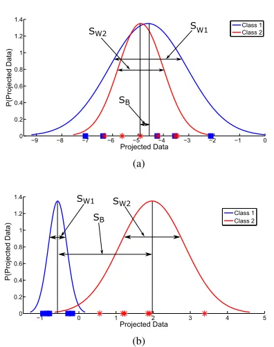
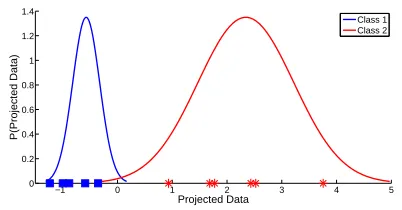
Fig. 4. Probability density function of the projected data of the first example, (a) the projected data onV1, (b) the projected data onV2.
Figure (4) illustrates aprobability density function
(pdf) graph of the projected data (yi) on the two
eigen-vectors (V1andV2). A comparison of the two
eigenvec-tors reveals the following :
– The data of each class is completely discrimi-nated when it is projected on the second eigen-vector (see Fig. (4)(b)) than the first one (see Fig. (4a)). In other words, the second eigenvector maximizes the between-class variance more than the first one.
– The within-class variance (i.e. the variance be-tween the same class samples) of the two classes are minimized when the data are projected on the second eigenvector. As shown in Fig. ((4)(b)), the within-class variance of the first class is small compared with Fig. ((4)(a)).
3.2. Class-Dependent Method
In this section, the LDA space is calculated using the class-dependent method. As mentioned in Sect. 2.5, the class-dependent method aims to calculate a sepa-rate transformation matrix (Wi) for each class.
The within-class variance for each class (SWi(2×
2)) is calculated as in class-independent method. The transformation matrix (Wi) for each class is then cal-culated as follows,Wi=SW−1iSB. The values of the two
transformation matrices (W1 andW2) will be as
fol-lows:
W1=SW−11SB=
10.00 8.00 8.00 7.20
−1
7.58 −7.27
−7.27 6.98
=
0.90 −1.00
−1.00 1.25
7.58 −7.27
−7.27 6.98
=
14.09 −13.53
−16.67 16.00
(28) Similarly,W2is calculated as follows:
W2=
1.70 −1.63
−1.50 1.44
(29) The eigenvalues (λi) and eigenvectors (Vi) for each
transformation matrix (Wi) are calculated, and the val-ues of the eigenvalval-ues and eigenvectors are shown be-low.
λω1=
0.00 0.00 0.00 30.01
andVω1=
−0.69 0.65
−0.72 −0.76
(30)
λω2=
3.14 0.00 0.00 0.00
andVω2=
0.75 0.69
−0.66 0.72
(31) whereλωiandVωi represent the eigenvalues and
eigen-vectors of theithclass, respectively.
From the results shown (above) it can be seen that, the second eigenvector of the first class (Vω{12}) has cor-responding eigenvalue more than the first one; thus, the second eigenvector is used as a lower dimensional space for the first class as follows, y1=ω1∗V
{2} ω1 , wherey1 represents the projection of the samples of
the first class. While, the first eigenvector in the second class (Vω{21}) has corresponding eigenvalue more than the second one. Thus,Vω{21}is used to project the data of the second class as follows,y2=ω2∗V
{1}
ω2 , wherey2 represents the projection of the samples of the second class. The values ofy1andy2will be as follows:
y1=
−0.88
−1.00
−0.35
−1.24
−0.59
andy2=
1.68 3.76 2.43 0.93 1.77 2.53
[image:11.595.308.517.172.327.2] [image:11.595.307.519.392.475.2]Figure (5) shows a pdf graph of the projected data (i.e.y1andy2) on the two eigenvectors (V
{2} ω1 andV
{1} ω2 ) and a number of findings are revealed the following:
– First, the projection data of the two classes are efficiently discriminated.
– Second, the within-class variance of the projected samples is lower than the within-class variance of the original samples.
−1 0 1 2 3 4 5
0 0.2 0.4 0.6 0.8 1 1.2 1.4
Projected Data
P(Projected Data)
[image:12.595.70.271.249.354.2]Class 1 Class 2
Fig. 5. Probability density function (pdf) of the projected data using class-dependent method, the first class is projected onVω{12}, while the second class is projected onVω{21}.
3.3. Discussion
In these two numerical examples, the LDA space is calculated using class-dependent and class-independent methods.
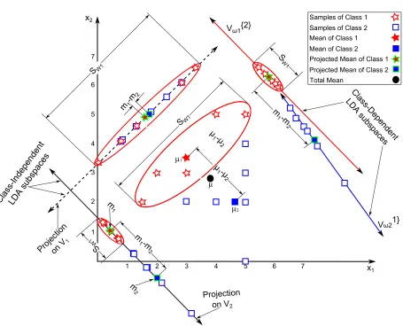
Figure (6) shows a further explanation of the two methods as following:
– Class-Independent: As shown from the figure, there are two eigenvectors,V1(dotted black line)
andV2(solid black line). The differences between
the two eigenvectors are as follows:
∗ The projected data on the second eigenvec-tor (V2) which has the highest corresponding
eigenvalue will discriminate the data of the two classes better than the first eigenvector. As shown in the figure, the distance between the projected meansm1−m2which representsSB,
increased when the data are projected onV2
thanV1.
∗ The second eigenvector decreases the within-class variance much better than the first eigen-vector. Figure (6) illustrates that the within-class variance of the first within-class (SW1) was much smaller when it was projected onV2thanV1. ∗ As a result of the above two findings,V2is used
to construct the LDA space.
– Class-Dependent: As shown from the figure, there are two eigenvectors, Vω{12} (red line) and V
{1} ω2 (blue line), which represent the first and second classes, respectively. The differences between the two eigenvectors are as following:
∗ Projecting the original data on the two eigen-vectors discriminates between the two classes. As shown in the figure, the distance between the projected meansm1−m2is larger than the
distance between the original meansµ1−µ2. ∗ The within-class variance of each class is
de-creased. For example, the within-class variance of the first class (SW1) is decreased when it is projected on its corresponding eigenvector.
∗ As a result of the above two findings,Vω{21}and Vω{21}are used to construct the LDA space. – Class-Dependent vs. Class-Independent: The two
LDA methods are used to calculate the LDA space, but a class-dependent method calculates separate lower dimensional spaces for each class which has two main limitations: (1) it needs more CPU time and calculations more than class-independent method; (2) it may lead toSSS prob-lem because the number of samples in each class affects the singularity ofSWi
2.
These findings reveal that the standard LDA technique used the class-independent method rather than using the class-dependent method.
4. Main Problems of LDA
Although LDA is one of the most common data re-duction techniques, it suffers from two main problems: the Small Sample Size (SSS) and linearity problems. In the next two subsections, these two problems will be explained, and some of the state-of-the-art solutions are highlighted.
4.1. Linearity problem
LDA technique is used to find a linear transforma-tion that discriminates between different classes. How-ever, if the classes are non-linearly separable, LDA can not find a lower dimensional space. In other words, LDA fails to find the LDA space when the discrimina-tory information are not in the means of classes.
1 2 3 4 5 6
1 2 3 4 5 6
x2
µ1
Vω21}
Vω1{2}
SamplesPofPClassP1
Class-D
epende
ntP LDAPsubsp
aces
Proj ectionP
onPV
1
µ2
µ
SamplesPofPClassP2
7 7
x1 Class-Ind
epende ntP
LDAPsubsp aces
SW1
S W1
S W1 SW1
m 1-m
2 m
1
m 2
m1-m
2
ProjectionP onPV2
m 1-m
2 µ
1-µ 2
µ 1-µ
2
MeanPofPClassP1 MeanPofPClassP2
[image:13.595.63.518.115.492.2]ProjectedPMeanPofPClassP1 ProjectedPMeanPofPClassP2 TotalPMean
Fig. 6. Illustration of the example of the two different methods of LDA methods. The blue and red lines represent the first and second eigenvectors of the class-dependent approach, respectively, while the solid and dotted black lines represent the second and first eigenvectors of class-indepen-dent approach, respectively.
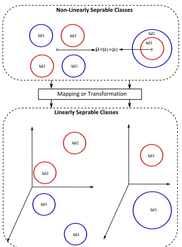
ure (7) shows how the discriminatory information does not exist in the mean, but in the variance of the data. This is because the means of the two classes are equal. The mathematical interpretation for this problem is as follows: if the means of the classes are approximately equal, so theSBandW will be zero. Hence, the LDA
space cannot be calculated.
One of the solutions of this problem is based on the transformation concept, which is known as a kernel methods or functions[50,3]. Figure (7) illustrates how the transformation is used to map the original data into a higher dimensional space; hence, the data will be lin-early separable, and the LDA technique can find the lower dimensional space in the new space. Figure (8) graphically and mathematically shows how two
non-separable classes in one-dimensional space are trans-formed into a two-dimensional space (i.e. higher di-mensional space); thus, allowing linear separation.
The kernel idea is applied in Support Vector Ma-chine (SVM) [49,66,69] Support Vector Regression (SVR)[58], PCA [51], and LDA [50]. Letφrepresents
a nonlinear mapping to the new feature space
Z
. The transformation matrix (W) in the new feature space (Z
) is calculated as in Equation (33).F(W) =max
WTSφBW WTSφ
WW
µ= =µ1µ2
x x
ω1
Mapping or Transformation Non-Linearly Seprable Classes
Linearly Seprable Classes
ω1 ω1
ω1
ω1
ω1 ω2
ω2
ω2
ω2
ω2
[image:14.595.315.510.101.392.2]ω2
Fig. 7. Two examples of two non-linearly separable classes, top panel shows how the two classes are non-separable, while the bot-tom shows how the transformation solves this problem and the two classes are linearly separable.
SφB=
c
∑
i=1
ni(µφi−µφ)(µφ
i −µφ)T (34)
SWφ =
c
∑
j=1 nj
∑
i=1
(φ{xi j} −µφj)(φ{xi j} −µφj)
T (35)
where µφi = n1
i∑
ni
i=1φ{xi} and µφ = 1 N∑
N
i=1φ{xi} =
∑ci=1 ni
Nµ φ i
Thus, in kernel LDA, all samples are transformed non-linearly into a new space
Z
using the functionφ. In other words, theφfunction is used to map the original features into
Z
space by creating a nonlin-ear combination of the original samples using a dot-products of it [3]. There are many types of kernel functions to achieve this aim. Examples of these func-tion include Gaussian or Radial Basis Funcfunc-tion (RBF),K(xi,xj) =exp(−||xi−xj||2/2σ2), whereσis a
posi-tive parameter, and the polynomial kernel of degreed,
K(xi,xj) = (xi,xj+c)d, [3,51,72,29].
1 2
Mapping
0 1 2 3 4
-1 -2
1 2
0 -1 -2
X
Φ(x)=(x,x2)=(z
1,z2)=Z
z2
z1
(1)→ (1,1) (-1)→(-1,1)
(2)→ (2,4) (-2)→(-2,4) Samples are
Non-linearly Seprable
Samples are
linearly Seprable
Class 1 Class 2
Fig. 8. Example of kernel functions, the samples lie on the top panel (X) which are represented by a line (i.e. one-dimensional space) are non-linearly separable, where the samples lie on the bottom panel (Z) which are generated from mapping the samples of the top space are linearly separable.
4.2. Small Sample Size Problem 4.2.1. Problem Definition
Singularity, Small Sample Size (SSS), or under-sampled problem is one of the big problems of LDA technique. This problem results from high-dimensional pattern classification tasks or a low number of train-ing samples available for each class compared with the dimensionality of the sample space [30,38,85,82].
TheSSS problem occurs when theSW is singular3.
The upper bound of the rank4of SW is N−c, while
the dimension ofSW isM×M[38,17]. Thus, in most
casesM >>N−cwhich leads to SSS problem. For example, in face recognition applications, the size of the face image my reach to 100×100=10000 pixels, which represent high-dimensional features and it leads to a singularity problem.
3A matrix is singular if it is square, does not have a matrix
in-verse, the determinant is zeros; hence, not all columns and rows are independent
4The rank of the matrix represents the number of linearly
[image:14.595.73.260.124.377.2]4.2.2. Common Solutions to SSS Problem:
There are many studies that proposed many solu-tions for this problem; each has its advantages and drawbacks.
– Regularization (RLDA): In regularization method, the identity matrix is scaled by multiplying it by a regularization parameter (η>0) and adding it to the within-class matrix to make it non-singular [18,38,82,45]. Thus, the diagonal components of the within-class matrix are biased as follows,
SW =SW+ηI. However, choosing the value of
the regularization parameter requires more tuning and a poor choice for this parameter can degrade the performance of the method [38,45]. Another problem of this method is that the parameterηis
just added to perform the inverse ofSW and has
no clear mathematical interpretation [38,57].
– Sub-space: In this method, a non-singular inter-mediate space is obtained to reduce the dimen-sion of the original data to be equal to the rank of SW; hence, SW becomes full-rank5, and then SW can be inverted. For example, Belhumeur et
al. [4] used PCA, to reduce the dimensions of the original space to be equal toN−c(i.e. the upper bound of the rank ofSW). However, as reported
in [22], losing some discriminant information is a common drawback associated with the use of this method.
– Null Space:There are many studies proposed to remove the null space ofSWto makeSW full-rank;
hence, invertible. The drawback of this method is that more discriminant information is lost when the null space ofSW is removed, which has a
neg-ative impact on how the lower dimensional space satisfies the LDA goal [83].
Four different variants of the LDA technique that are used to solve the SSS problem are introduced as fol-lows:
PCA + LDA technique: In this technique, the orig-inal d-dimensional features are first reduced to h-dimensional feature space using PCA, and then the LDA is used to further reduce the features to k-dimensions. The PCA is used in this technique to re-duce the dimensions to make the rank of SWis N−c as reported in [4]; hence, the SSS problem is addressed. However, the PCA neglects some discriminant infor-mation, which may reduce the classification perfor-mance [57,60].
5Ais a full-rank matrix if all columns and rows of the matrix are
independent, (i.e. rank(A)=# rows=#cols) [23]
Direct LDA technique: Direct LDA (DLDA) is one of the well-known techniques that are used to solve the SSS problem. This technique has two main steps [83]. In the first step, the transformation matrix, W , is com-puted to transform the training data to the range space of SB. In the second step, the dimensionality of the transformed data is further transformed using some regulating matrices as in Algorithm 4. The benefit of the DLDA is that there is no discriminative features are neglected as in PCA+LDA technique [83].
Regularized LDA technique: In the Regularized LDA (RLDA), a small perturbation is add to theSW matrix
to make it non-singular as mentioned in [18]. This reg-ularization can be applied as follows:
(SW+ηI)−1SBwi=λiwi (36) whereηrepresents a regularization parameter. The di-agonal components of theSWare biased by adding this
small perturbation [18,13]. However, the regularization parameter need to be tuned and poor choice of it can degrade the generalization performance [57].
Null LDA technique: The aim of the NLDA technique is to find the orientation matrix W , and this can be achieved using two steps. In the first step, the range space of the SW is neglected, and the data are projected only on the null space of SW as follows, SWW =0. In the second step, the aim is to search for W that satis-fies SBW =0and maximizes|WTSBW|. The higher di-mensionality of the feature space may lead to compu-tational problems. This problem can be solved by (1) using the PCA technique as a pre-processing step, i.e. before applying the NLDA technique, to reduce the di-mension of feature space to be N−1; by removing the null space of ST =SB+SW [57], (2) using the PCA technique before the second step of the NLDA tech-nique [54]. Mathematically, in the Null LDA (NLDA) technique, the h column vectors of the transformation matrix W = [w1,w2, . . . ,wh] are taken to be the null space of the SW as follows, wTiSWwi=0,∀i=1. . .h, where wTiSBwi6=0. Hence, M−(N−c)linearly inde-pendent vectors are used to form a new orientation ma-trix, which is used to maximize|WTSBW|subject to the constraint|WTSWW|=0as in Equation (37).
W =arg max |WTS
WW|=0
5. Applications of the LDA technique
In many applications, due to the high number of fea-tures or dimensionality, the LDA technique have been used. Some of the applications of the LDA technique and its variants are described as follows:
5.1. Biometrics Applications
Biometrics systems have two main steps, namely, feature extraction (including pre-processing steps) and recognition. In the first step, the features are extracted from the collected data, e.g. face images, and in the second step, the unknown samples, e.g. unknown face image, is identified/verified. The LDA technique and its variants have been applied in this application. For example, in [83,10,41,75,20,68], the LDA technique have been applied on face recognition. Moreover, the LDA technique was used in Ear [84], fingerprint [44], gait [5], and speech [24] applications. In addition, the LDA technique was used with animal biometrics as in [65,19].
5.2. Agriculture Applications
In agriculture applications, an unknown sample can be classified into a pre-defined species using computa-tional models [64]. In this application, different vari-ants of the LDA technique was used to reduce the di-mension of the collected features as in [9,26,46,21,64, 63].
5.3. Medical Applications
In medical applications, the data such as the DNA microarray data consists of a large number of features or dimensions. Due to this high dimensionality, the computational models need more time to train their models, which may be infeasible and expensive. More-over, this high dimensionality reduces the classifica-tion performance of the computaclassifica-tional model and in-creases its complexity. This problem can be solved us-ing LDA technique to construct a new set of features from a large number of original features. There are many papers have been used LDA in medical applica-tions [54,52,53,16,39,55,8].
6. Packages
In this section, some of the available packages that are used to compute the space of LDA variants. For example, WEKA6 is a well-known Java-based data
mining tool with open source machine learning soft-ware such as classification, association rules, regres-sion, pre-processing, clustering, and visualization. In WEKA, the machine learning algorithms can be ap-plied directly on the dataset or called from person’s Java code. XLSTAT7is another data analysis and sta-tistical package for Microsoft Excel that has a wide variety of dimensionality reduction algorithms includ-ing LDA. dChip8package is also used for visualiza-tion of gene expression and SNP microarray including some data analysis algorithms such as LDA, cluster-ing, and PCA. LDA-SSS9is a Matlab package, and it contains several algorithms related to the LDA tech-niques and its variants such as DLDA, PCA+LDA, and NLDA. MASS10 package is based on R, and it has
functions that are used to perform linear and quadratic discriminant function analysis. Dimensionality reduc-tion11package is mainly written in Matlab, and it has a number of dimensionality reduction techniques such as ULDA, QLDA, and KDA. DTREG12is a software package that is used for medical data and modeling business, and it has several predictive modeling meth-ods such as LDA, PCA, linear regression, and decision trees.
7. Experimental Results and Discussion
In this section, two experiments were conducted to illustrate: (1) how the LDA is used for different appli-cations, (2) what is the relation between its parame-ter (Eigenvectors) and the accuracy of a classification problem, (3) when theSSSproblem could appear and a method for solving it.
6http:/www.cs.waikato.ac.nz/ml/weka/ 7http://www.xlstat.com/en/
7.1. Experimental Setup
This section gives an overview of the databases, the platform, and the machine specification used to conduct our experiments. Different biometric datasets were used in the experiments to show how the LDA using its parameter behaves with different data. These datasets are described as follows:
– ORL dataset13 face images dataset (Olivetti Re-search Laboratory, Cambridge) [48], which con-sists of 40 distinct individuals, was used. In this dataset, each individual has ten images taken at different times and varying light conditions. The size of each image is 92×112.
– Yale dataset14 is another face images dataset which contains 165 grey scale images in GIF for-mat of 15 individuals [78]. Each individual has 11 images in different expressions and configura-tion: center-light, happy, left-light, with glasses, normal, right-light, sad, sleepy, surprised, and a wink.
– 2D ear dataset (Carreira-Perpinan,1995)15images dataset [7] was used. The ear data set consists of 17 distinct individuals. Six views of the left pro-file from each subject were taken under a uniform, diffuse lighting.
In all experiments,k-fold cross-validation tests have used. Ink-fold cross-validation, the original samples of the dataset were randomly partitioned intoksubsets of (approximately) equal size and the experiment is runk
times. For each time, one subset was used as the testing set and the otherk−1 subsets were used as the train-ing set. The average of thekresults from the folds can then be calculated to produce a single estimation. In this study, the value ofkwas set to 10.
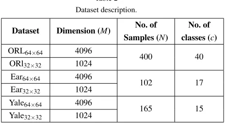
The images in all datasets resized to be 64×64 and 32×32 as shown in Table (2). Figure (9) shows sam-ples of the used datasets and Table (2) shows a descrip-tion of the datasets used in our experiments.
In all experiments, to show the effect of the LDA with its eigenvector parameter and itsSSSproblem on the classification accuracy, the Nearest Neighbour clas-sifier was used. This clasclas-sifier aims to classify the test-ing image by compartest-ing its position in the LDA space with the positions of training images. Furthermore, class-independent LDA was used in all experiments.
13http://www.cam-orl.co.uk
14http://vision.ucsd.edu/content/yale-face-database
[image:17.595.299.531.295.422.2]15http://faculty.ucmerced.edu/mcarreira-perpinan/software.html
Fig. 9. Samples of the first individual in: ORL face dataset (top row); Ear dataset (middle row), and Yale face dataset (bottom row).
Table 2 Dataset description.
Dataset Dimension (M) No. of
Samples (N)
No. of
classes (c)
ORL64×64 4096
400 40
ORl32×32 1024
Ear64×64 4096
102 17
Ear32×32 1024
Yale64×64 4096
165 15
Yale32×32 1024
Moreover, Matlab Platform (R2013b) and using a PC with the following specifications: Intel(R) Core(TM) i5-2400 CPU @ 3.10 GHz and 4.00 GB RAM, under Windows 32-bit operating system were used in our ex-periments.
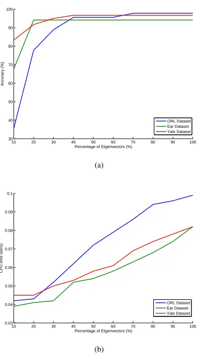
7.2. Experiment on LDA Parameter (Eigenvectors)
The aim of this experiment is to investigate the re-lation between the number of eigenvectors used in the LDA space, and the classification accuracy based on these eigenvectors and the required CPU time for this classification.
investi-10 20 30 40 50 60 70 80 90 100 30
40 50 60 70 80 90 100
Percentage of EIgenvectors (%)
Accuracy (%)
ORL Dataset Ear Dataset Yale Dataset
(a)
10 20 30 40 50 60 70 80 90 100 0.03
0.04 0.05 0.06 0.07 0.08 0.09 0.1
Percentage of EIgenvectors (%)
CPU time (secs)
ORL Dataset Ear Dataset Yale Dataset
[image:18.595.312.512.112.280.2](b)
Fig. 10. Accuracy and CPU time of the LDA techniques using dif-ferent percentages of eigenvectors, (a) Accuracy (b) CPU time.
gate these issue, three datasets listed in Table (2) (i.e. ORL32×32, Ear32×32, Yale32×32), were used. Moreover,
seven, four, and eight images from each subject in the ORL, ear, Yale datasets, respectively, are used in this experiment. The results of this experiment are pre-sented in Fig. (10).
From Fig. (10) it can be noticed that the accu-racy and CPU time are proportional with the number of eigenvectors which are used to construct the LDA space. Thus, the choice of using LDA in a specific ap-plication should consider a trade-off between these fac-tors. Moreover, from Fig. (10a), it can be remarked that when the number of eigenvectors used in computing the LDA space was increased, the classification accu-racy was also increased to a specific extent after which the accuracy remains constant. As seen in Fig. (10a), this extent differs from application to another. For ex-ample, the accuracy of the ear dataset remains
con-5 10 15 20 25 30 35 40 0
0.1 0.2 0.3 0.4 0.5 0.6 0.7
The Index of the Eignvector
Weight of the Eigenvector
ORL Dataset Ear Dataset Yale Dataset
Fig. 11. The robustness of the first 40 eigenvectors of the LDA tech-nique using ORL32×32, Ear32×32, and Yale32×32datasets.
stant when the percentage of the used eigenvectors is more than 10%. This was expected as the eigenvec-tors of the LDA space are sorted according to their ro-bustness (see Sect. 2.6). Similarly, in ORL and Yale datasets the accuracy became approximately constant when the percentage of the used eigenvectors is more than 40%. In terms of CPU time, Fig. (10b) shows the CPU time using different percentages of the eigenvec-tors. As shown, the CPU time increased dramatically when the number of eigenvectors increases.
Fig. (11) shows the weights16 of the first 40 eigen-vectors which confirms our findings. From these re-sults, we can conclude that the high order eigenvectors of the data of each application (the first 10 % of ear database and the first 40 % of ORL and Yale datasets) are robust enough to extract and save the most discrim-inative features which are used to achieve a good accu-racy.
These experiments confirmed that increasing the number of eigenvectors will increase the dimension of the LDA space; hence, CPU time increases. Conse-quently, the amount of discriminative information and the accuracy increases.
7.3. Experiments on the Small Sample Size problem
The aim of this experiment is to show when the LDA is subject to theSSSproblem and what are the methods that could be used to solve this problem. In this experi-ment, PCA-LDA [4] and Direct-LDA [83,22] methods 16The weight of the eigenvector represents the ratio of its
cor-responding eigenvalue (λi) to the total of all eigenvalues (λi,i=
1,2, . . . ,k) as follows, λi
[image:18.595.74.271.130.482.2]are used to address theSSSproblem. A set of exper-iments was conducted to show how the two methods interact with theSSSproblem, including the number of samples in each class, the total number of classes used, and the dimension of each sample.
As explained in Sect. 4, using LDA directly may lead to the SSS problem when the dimension of the samples are much higher than the total number of sam-ples. As shown in Table (2), the size of each image or sample of the ORL dataset is64×64is 4096 and the
to-tal number of samples is 400. The mathematical inter-pretation of this point shows that the dimension ofSW
isM×M, while the upper bound of the rank ofSW is N−c[79,82]. Thus, all the datasets which are reported in Table (2) lead to singularSW.
To address this problem, PCA-LDA and direct-LDA methods were implemented. In the PCA-LDA method, PCA is first used to reduce the dimension of the origi-nal data to makeSW full-rank, and then standard LDA can be performed safely in the subspace ofSW as in Al-gorithm (3). For more details of the PCA-LDA method are reported in [4]. In the direct-LDA method, the null-space ofSW matrix is removed to makeSW full-rank,
then standard LDA space can be calculated as in Al-gorithm (4). More details of direct-LDA methods are found in [83].
Table (2) illustrates various scenarios designed to test the effect of different dimensions on the rank ofSW
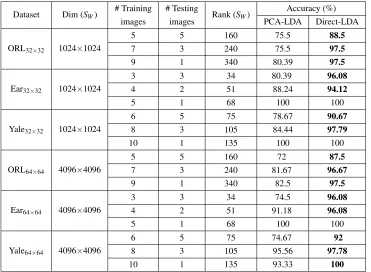
and the accuracy. The results of these scenarios using both PCA-LDA and direct-LDA methods are summa-rized in Table (3).
As summarized in Table (3), the rank ofSW is very
small compared to the whole dimension ofSW; hence,
the SSS problem occurs in all cases. As shown in Table (3), using the PCA-LDA and the Direct-LDA, the SSS problem can be solved and the Direct-LDA method achieved results better than PCA-LDA because as reported in [83,22], Direct-LDA method saves ap-proximately all important information for classifica-tion while the PCA in PCA-LDA method saves the in-formation with high variance.
8. Conclusions
In this paper, the definition, mathematics, and im-plementation of LDA were presented and explained. The paper aimed to give low-level details on how the LDA technique can address the reduction problem by extracting discriminative features based on maximiz-ing the ratio between the between-class variance,SB,
Algorithm 3.: PCA-LDA.
1: Read the training images (X ={x1,x2, . . . ,xN}),
wherexi(ro×co)represents theithtraining image, roandcorepresent the rows (height) and columns (width) ofxi, respectively,N represents the total
number of training images.
2: Convert all images in vector representation Z = {z1,z2, . . . ,zN}, where the dimension ofZ isM×
1,M=ro×co.
3: calculate the mean of each classµi, total mean of
all dataµ, between-class matrix SB(M×M), and
within-class matrix SW(M×M) as in Algorithm
(1, Step(2-5)).
4: Use the PCA technique to reduce the dimension of
Xto be equal to or lower thanr, whererrepresents the rank ofSW, as follows:
XPCA=UTX (38)
where,U∈
R
M×ris the lower dimensional spaceof the PCA andXPCArepresents the projected data
on the PCA space.
5: Calculate the mean of each classµi, total mean of
all data µ, between-class matrix SB, and
within-class matrix SW of XPCA as in Algorithm (1,
Step(2-5)).
6: CalculateW as in Equation (7) and then calculate the eigenvalues (λ) and eigenvectors (V) of theW
matrix.
7: Sorting the eigenvectors in descending order ac-cording to their corresponding eigenvalues. The firstkeigenvectors are then used as a lower dimen-sional space (Vk).
8: The original samples (X) are first projected on the PCA space as in Equation (38). The projection on the LDA space is then calculated as follows:
XLDA=VkTXPCA=VkTUTX (39)
whereXLDArepresents the final projected on the
LDA space.
and within-class variance,SW, thus discriminating
be-tween different classes. To achieve this aim, the paper followed the approach of not only explaining the steps of calculating theSB, andSW (i.e. the LDA space) but
Table 3
Accuracy of the PCA-LDA and direct-LDA methods using the datasets listed in Table (2).
Dataset Dim (SW)
# Training images
# Testing
images Rank (SW)
Accuracy (%) PCA-LDA Direct-LDA
ORL32×32 1024×1024
5 5 160 75.5 88.5
7 3 240 75.5 97.5
9 1 340 80.39 97.5
Ear32×32 1024×1024
3 3 34 80.39 96.08
4 2 51 88.24 94.12
5 1 68 100 100
Yale32×32 1024×1024
6 5 75 78.67 90.67
8 3 105 84.44 97.79
10 1 135 100 100
ORL64×64 4096×4096
5 5 160 72 87.5
7 3 240 81.67 96.67
9 1 340 82.5 97.5
Ear64×64 4096×4096
3 3 34 74.5 96.08
4 2 51 91.18 96.08
5 1 68 100 100
Yale64×64 4096×4096
6 5 75 74.67 92
8 3 105 95.56 97.78
10 1 135 93.33 100
The bold values indicate that the corresponding methods obtain best performances
and graphically illustrated to explain how the LDA space using the two methods can be constructed. In all examples, the mathematical interpretation of the robustness and the selection of the eigenvectors as well the data projection were detailed and discussed. Also, LDA common problems (e.g. the SSS and lin-earity) were mathematically explained using graphi-cal examples, then their state-of-the-art solutions are highlighted. Moreover, a detailed implementation of LDA applications was presented. Using three standard datasets, a number of experiments were conducted to (1) investigate and explain the relation between the number of eigenvectors and the robustness of the LDA space, (2) to practically show when the SSS problem occurs and how it can be addressed.
References
[1] S. Balakrishnama and A. Ganapathiraju. Linear discriminant analysis-a brief tutorial. Institute for Signal and information Processing, 1998.
[2] E. Barshan, A. Ghodsi, Z. Azimifar, and M. Z. Jahromi. Su-pervised principal component analysis: Visualization, classifi-cation and regression on subspaces and submanifolds.Pattern Recognition, 44(7):1357–1371, 2011.
[3] G. Baudat and F. Anouar. Generalized discriminant analysis using a kernel approach. Neural computation, 12(10):2385– 2404, 2000.
[4] P. N. Belhumeur, J. P. Hespanha, and D. Kriegman. Eigenfaces vs. fisherfaces: Recognition using class specific linear projec-tion.IEEE Transactions on Pattern Analysis and Machine In-telligence, 19(7):711–720, 1997.
[5] N. V. Boulgouris and Z. X. Chi. Gait recognition using radon transform and linear discriminant analysis.IEEE transactions on image processing, 16(3):731–740, 2007.
[6] M. Bramer. Principles of data mining. Springer, Second Edi-tion, 2013.
[7] M. Carreira-Perpinan. Compression neural networks for fea-ture extraction: Application to human recognition from ear im-ages. MS thesis, Faculty of Informatics, Technical University of Madrid, Spain, 1995.
[8] H.-P. Chan, D. Wei, M. A. Helvie, B. Sahiner, D. D. Adler, M. M. Goodsitt, and N. Petrick. Computer-aided classification of mammographic masses and normal tissue: linear discrimi-nant analysis in texture feature space.Physics in medicine and biology, 40(5):857, 1995.
[9] L. Chen, N. C. Carpita, W.-D. Reiter, R. H. Wilson, C. Jeffries, and M. C. McCann. A rapid method to screen for cell-wall mu-tants using discriminant analysis of fourier transform infrared spectra.The Plant Journal, 16(3):385–392, 1998.