Simulation of Dynamic Propagation of Electromagnetic Wave in Microwave Passive Components Using Open Source Finite Element Software

(1)

International Journal of Emerging Technology and Advanced Engineering

Website: www.ijetae.com (ISSN 2250-2459,ISO 9001:2008Certified Journal, Volume 3, Issue 8, August 2013)

44

Simulation of Dynamic Propagation of Electromagnetic Wave

in Microwave Passive Components Using Open Source Finite

Element Software

Ndagije Charles

Faculty of applied fundamental sciences, Institute of Higher Education (INES) Ruhengeri, P.O. Box 155 Ruhengeri (Rwanda)

Abstract- Computer modeling and simulations of physical processes plays an important role in teaching engineering courses, in particular for difficult courses like electromagnetic and microwave engineering. In this paper we analyze the electromagnetic wave propagation in different passive microwave components such as rectangular metallic waveguides, bend waveguides and tee junctions using open source finite element software from the OneLab project: Gmsh and GetDP. The resulting fully parameterized finite element models have been used in teaching the course of microwave communication at the National University of Rwanda and have played an important role to facilitate the students’ understanding of the course.

Keywords: Simulation, Maxwell’s equations, waveguide, tee junctions, finite element method, electromagnetic field, weak formulation, discrete formulation, Galerkin Method.

I. INTRODUCTION

Many universities, especially those in the developing countries, suffer from the lack of (often expensive) laboratory equipment for conducting practical courses on important engineering topics, like electromagnetic and microwave engineering. One way to improve the manner those courses are taught is to use simulation techniques.

It was realized that Modeling and simulation can help the students to better understand such courses without using hardware equipment. In addition, successful modeling and simulation requires a very good understanding of the subject, some mathematical knowledge and computer skills which all contribute to the overall training of engineering students. Electromagnetic wave propagation in microwave passive components is described by inhomogeneous partial differential equations (PDEs) that are often hard or impossible to solve analytically, which complicates the analysis of that process. In this paper we propose to set up parametric finite element models to compute the propagation of electromagnetic wave in metallic waveguides and tee junctions.

Such structures are widely used in telecommunication for ultrahigh and super high frequencies. Modeling such waveguides requires the solution of Maxwell’s equations, which can be obtained numerically by using the finite element method [14], [11]. We propose to evaluate the time-dependent solution of Maxwell’s equations in these waveguides. The main advantages of using the finite element method for analyzing the wave propagation in the waveguides is that it makes it easy to visualize the pattern of wave propagation in those structures while by using analytical methods it is only possible to determine the critical frequency and the condition for which the wave can be able to propagate in simple geometrical configurations. In the context of engineering courses such numerical simulations can help to clearly display wave patterns and other relevant physical quantities (e.g. S matrix) without using laboratory equipment. In addition, by building fully parameterized models (where the dimensions, materials, operating frequency,…can be changed interactively) the simulations can help to understand experimental measurements and to design new applications.

The results of this work have been used in teaching the course of microwave communication at the National University of Rwanda in 2010-2011, 2011-2012 and 2012-2013 to the population of about 40 students. The developed parametric models helped the students to easily understand that by changing the parameters of the wave guide the operating frequencies are also changing as well as the propagation characteristics of corresponding modes in waveguide.

(2)

International Journal of Emerging Technology and Advanced Engineering

45

II. MATHEMATICAL FORMULATION OF THE PROBLEM

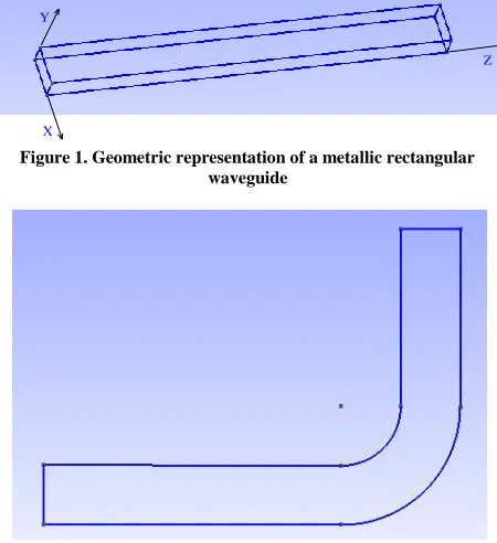
[image:2.612.330.559.138.295.2]

The dynamic simulation of electromagnetic wave in those structures is analyzed by solving Maxwell’s equation with considering boundary conditions. Let start by analyzing simple rectangular waveguide, bend waveguide and tee-junctions (see Figure 1, 2, 3and 4).

[image:2.612.56.281.225.471.2]

Figure 1. Geometric representation of a metallic rectangular waveguide

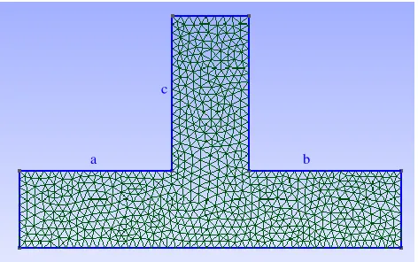
Figure 2. Geometric representation of a section of a bend rectangular waveguide

Figure 3: Geometric representation of a E-plane tee junction

Figure 4: Geometric representation of a microwave Y circulator

Maxwell’s equations in linear media read:

.

,

.

0,

(1)

,

E

B

H

E

t

E

H

j

t









 



 





_{  }





_







 



_



Where

E

(

V

/

m

)



is the electrical field intensity ,

)

/

(

Coul

m

3



is the electrical charge density,



is the permittivity of the medium,

B

(

Web

/

m

2

)



is magnetic flux density,



is the permeability of the medium,

)

/

(

A

m

H



is the magnetic field intensity,



j

(

A

/

m

2

)

is the conduction current density. If the considered medium

is the air, the permittivity becomes



₀, and the permeability

becomes



₀, where₀ 8.854.1012Farad/mand

m henry/ 7 10 . 4

0

  

 .

By using the properties of vector analysis the system (1) of first order partial differential equations (PDEs) can be rewritten as the following second order equation:

t

j

t

E





















0 2

2 0

0





(2)

X Y

Z

a

b c

1

2

3

[image:2.612.51.289.506.650.2]

(3)

International Journal of Emerging Technology and Advanced Engineering

46

In general the current density

j



is a function of time

and space. In the cases that we are going to treat next we will assume that the metallic surfaces of the waveguide are

perfect conductors;

j



will thus represent only a source of the electromagnetic waves. The electrical field Emust satisfy the boundary conditions, i.e., its tangential components must be equal to zero on the waveguide surfaces, meaning that the following condition has to be satisfied [5]:

0 



E

n



, where

n



is the outgoing unit normal vector. Foreffective transmission of information in waveguide it is very important to know if the transmission channel is adequate referring to the frequency to transmit. In order to know which waves (modes) are able to propagate through a given wave guide, we need to compute the eigenfrequencies f[Hz] of the waveguide. This problem can be solved by using finite element method.

III. FINITE ELEMENT METHOD

The finite element method is a powerful computational technique which can help to approximate solutions to PDEs encountered in scientific and engineering applications [10].

With the finite element method the solution of PDEs is found by following different steps. The first step is the preprocessing which includes the definition of the geometric domain of the problem, the definition of elements type to use for domain discretization, the definition of material properties of the elements, and the definition of the physical constraints. The second step is the solution phase. During this step the finite element software assembles the governing algebraic equations in matrix form and computes the unknown values. This step requires the discrete formulation of the problem through the weak formulation of the problem (see section 5). For thediscrete formulation of the problem we used the Galerkin method [10], [7] as implemented in the open source software GetDP [2].

The last step of finite element method is the post processing which is focused on analysis and evaluation of the solution results. In this study this step was carried out by using the Gmsh open source software [1].

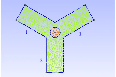
[image:3.612.329.563.138.301.2]

The next figures represent the discretization of the domains of resolution which are the rectangular waveguide, the section of a bend waveguide, the section of E-plane tee junction and the section of a waveguide Y circulator.

[image:3.612.326.567.330.497.2]

Figure 5: Discretized rectangular waveguide

Figure 6: Discretized bend waveguide

Figure 7: Discretized E-plane tee junction Y

X

Z

a b

[image:3.612.327.563.525.673.2]

(4)

International Journal of Emerging Technology and Advanced Engineering

[image:4.612.49.287.140.298.2]

47

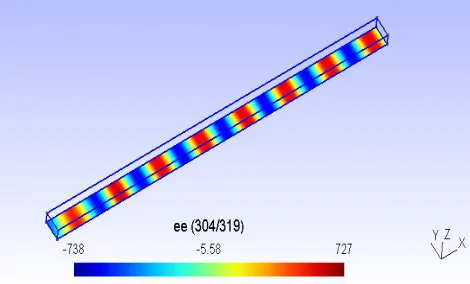
Figure 8: Discretized waveguide Y circulator

IV. WEAK FORMULATION OF THE PROBLEM

For the weak formulation of the problem, we used the method of weighted residual [10]. According to this

method, instead of solving (2) directly, we look for

E



such that

2

. 0 (3) 0 0 2 0

E j

E U d

t t                     













holds for appropriately chosen weight (test) functions U . By using the properties of vector analysis the equation (3) can be rewritten as follows:

2

.( ) . _{0 0} ₂ .

. 0 (4) 0

E

U A d U A d U d

t j U d t     _  _  _  _                           

Where A  E. By using the divergence theorem, the expression (4) becomes

                 



     d U t j d U t E d U E d n A U . . ) ).( ( ) ( ). ( 0 2 2 0 0              

Where





is a curve delimiting the surface



_{. By} using the property of vector analysis, we get

(U A n d). ( ) A n U d.( ) ( ) 0

         

 

,

because it is necessary to chose the weight function which

also satisfies the boundary conditions such thatn U 0.

Finally the integral in (4) can be written as follows:

(5) 0 . 0 . 2 2 0 0 ) ).( (                

 tUd

j d U t E d U E           

This expression represents the weak formulation of the problem.

V. DISCRETE FORMULATION OF THE PROBLEM

The discrete formulation consists in approximating the

electric field

E



using a finite number of shape functions

(basis functions)_{W j}:

1

(6)

N

E C W_j _j

j

 



The GetDP code uses so-called Whitney edge elements to approximate the electric field. In this case, the functions

W j have continuous tangential components across element borders, but discontinuous normal components and the coefficients _{C j} are the circulations of E along each

edge of the mesh.

N

is the total number of edges in the mesh. By using the Galerkin method, the weight functions

U are chosen identical to the form functionsW , i.e.,

, 1, 2, 3,... (7) k

U W k N .

Introducing (7 and (6) into (5) leads to a system of N linear equations: 0 . . 0 1 1 2 2 0

0 _ 

 _           _         



W d

t j d W t W C d W Curl W Curl C k N j N j k j j k j j          or (8) . . 0 1 2 2 0 0    _                      _        



W d

t j d W t W d W Curl W Curl C k N j k j k j j         

The expression (8) is the discrete formulation of the

problem. In this equation the unknowns are the values_{C j} .

1

2

(5)

International Journal of Emerging Technology and Advanced Engineering

48

The numerical resolution aims to find those values.

Once they are found the electrical field

E



can be obtained by using the expression (6).

VI. NUMERICAL SOLUTION

We tested the method by solving the equation (8) with

the presence of the source current



j

(

t

)

. ) (

. 0

1

2 2 0

0 _

 _

      

 

  

     

 

 _

   

 

 



W d

t t j d

W t W d

W Curl W Curl

C k

N j

k j k

j j

  

 



 



We first tested the case of wave propagation in rectangular waveguide. In this case we considered TM and TE-modes. For TM-modewe used homogeneous Dirichlet boundary condition while for TE-mode we used the Neuman boundary condition.

[image:5.612.328.563.133.210.2]

A. Electromagnetic wave propagation in rectangular waveguide

[image:5.612.50.279.237.277.2]

Figure 9: Propagation of TE-mode in rectangular waveguide

Figure 10: Propagation of TE-mode in rectangular waveguide (raised representation)

[image:5.612.331.559.368.511.2]

Figure 11: Propagation of TM-mode in rectangular waveguide

Figure 12: Propagation of TM-mode in rectangular waveguide (raised form)

[image:5.612.52.287.376.518.2]

B.Electromagnetic wave propagation in bend waveguide

Figure 13: Propagation of TM11 in bend rectangular waveguide

Figure 14: Raised view of propagation of TM11 in bend rectangular

[image:5.612.324.567.541.682.2] [image:5.612.52.287.545.636.2]

(6)

International Journal of Emerging Technology and Advanced Engineering

49

[image:6.612.50.287.149.292.2]

C. Types of tee junctions

Figure 15: Electrical field distribution in E-plane tee junction

[image:6.612.327.563.177.308.2]

In E-plan tee junction the electrical field is parallel to the arm port while for H-plane tee junction; it is perpendicular to the arm port as it is indicated on the next figure

Figure 16: Electrical field distribution in H-plane tee junction

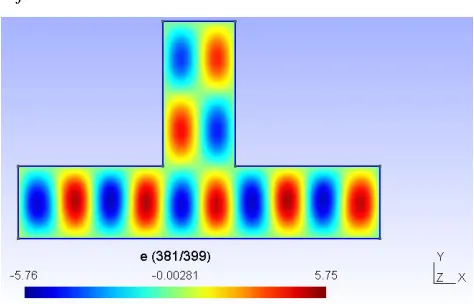
D. Electromagnetic wave propagation in E-plane tee junction

Figure 17: Propagation of electromagnetic wave in E-plane tee junction when the inputs are in collinear ports and in phase shift

[image:6.612.51.284.351.479.2]

In this case the inputs in collinear ports are in opposition of phase. When the inputs are in collinear ports, the output is in the arm port.

Figure 18: Propagation of electromagnetic wave in E-plane tee junction when the input is in arm port(c port)

When the input is in arm port, the output will be in collinear ports.

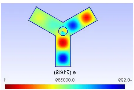
E. Waveguide Y circulator

The propagation of electromagnetic wave in waveguide Y circulator respects the following S- matrix

 

1 0 00 0 1 0 1 0

S 

















For this circulator , if the input is in port 1 the output will be in port 2, if the input is in port 2 the output will be in port 3, and finally if the input is in port 3 the output will be in port 1 [13]. The figures 19, 20, 21 are the illustrations of those types of electromagnetic wave propagation.

Figure 19: Wave propagation in a waveguide Y circulator when the input is in port 2

a b

[image:6.612.50.287.521.673.2] [image:6.612.331.559.543.696.2]

(7)

International Journal of Emerging Technology and Advanced Engineering

[image:7.612.57.278.138.300.2]

50

Figure 20: Wave propagation in a waveguide Y circulator when the

input is in port 3.

Figure 21: Wave propagation in a waveguide Y circulator when the input is in port 1

VII. CONCLUSION

In this study the electromagnetic wave propagation in rectangular waveguide, bend waveguide, E-plane tee junction and waveguide Y circulator has been described and simulated, by using the finite element method.

The found results were applied during the teaching of the course of microwave communication in third year electronics and communication systems at National University of Rwanda. It was demonstrated that the simulation techniques can facilitate not only the better understanding but also the better teaching of engineering courses especially when the equipments are not available.

One of the particular advantages of finite element method is its capacity of visualization of results which are sometimes an abstract concept.

This work is the continuity of our previous study which was focused only on mode description in rectangular waveguide [12].

REFERENCES

[1] C. Geuzaine and J.-F. Remacle, Gmsh. A three- dimensional finite element meshes generation with built-in pre-and post-processing facilities. International for Numerical Method in Engineering, Volume 79, Issue 11, pages 1909-1331, 2009. http://www.geuz.org/gmsh.

[2] Patrick Dular, Christophe Geuzaine, A general environment for the treatment of Discrete Problems, University of Liege, 1997-2011. http://www.geuz.org/gmsh.

[3] Granino A. KORN, Advanced dynamic –System simulation, Willey & Sons, Inc., Arizona, 2007.

[4] W. J. Minkowycz, E. M.Sparrow, J.Y. Murthy, Handbook of Numerical heat transfer, second edition, Willey &Sons, Inc., United States of America, 2006.

[5] Robert E. Collin, Foundations for Microwave Engineering, second edition, John Willey &Sons, Inc., New York, 2001

[6] G.R. Liu, S. S. Quek, The finite element method: A Practical course, Elsevier Science Ltd, Singapore, 2003.

[7] J.N. Reddy, An introduction to the finite element method, second edition, McGraw-Hill, In., Texas, 1993.

[8] Jean-Philippe Grivet, Méthodes numériques appliquées pour le scientifique et l’ingénieur, EDP Sciences, Paris 2009.

[9] Benoît Meys, Modélisation des champs électromagnétiques aux hyperfréquences par la méthode des éléments finis. Application au problème du chauffage diélectrique, Thèse présentée à la Faculté des sciences Appliquées, Université de Liège, 1999.

[10] David V. Hutton, Fundamental of finite element analysis, McGraw-Hill, New York, 2004.

[11] C. J. Reddy, Manohar D. Deshpande, C.R. Cockrell, and Fred B. Beck; Finite Element Method for Eigenvalue Problems in Electromagnetics, NASA Technical paper 3485, Virginia 23681-0001, 1994.

[12] C. Ndagije and C. Geuzaine, Simulation of Electromagnetic Field Distribution in Metallic Waveguides Using Open Source Finite Element Software, International Journal of Emerging Technology & Advanced Engineering, Volume3, Issue2, Page 91-98, February, 2013.

[13] Oussama Zahwe, Conception et Réalisation d’un Circulateur coplanaire à couche Magnétique de YIG en Bande X pour des Applications en Télécommunications ; Thèse pour obtenir le grade de Docteur de l’Université Jean Monnet de Saint-Etienne, 2009. [14] Matthew N. O. Sakidu, Numerical Techniques in Electromagnetics,

Second edition, CRC Press LLC, Florida, 2001. 1

2

[image:7.612.54.282.335.488.2]