Modelling the Effect of Subsurface Infrastructures on Ground Water Quantity Using GIS and MODFLOW

(1)

International Journal of Emerging Technology and Advanced Engineering

Website: www.ijetae.com (ISSN 2250-2459, ISO 9001:2008 Certified Journal, Volume 6, Issue 8, August 2016)

220

Modelling the Effect of Subsurface Infrastructures on Ground

Water Quantity Using GIS and MODFLOW

Reeya John.J

1

, Lilly.P

2

,

Ravikumar.G

3

1_{M.Tech.(EST) student, Dept. of Chemical Engg, A C Tech, Anna University, Chennai – 25, India} 2_{Assistant Professor in Civil Engg, Dept. of Civil Engg, MNM Jain Engineering College, Chennai, India}

3_{Professor in Civil Engg, Dept. of Civil Engg, Anna University, Chennai – 25, India} Abstract - Water is most essential for every living

organism. The water which is needed for the human life is fresh water and its only upto 2.8% of total water resources in earth .Of these fresh water, 2.2% is surface water and 0.6% is present in the form of ground water. As the population increases, the water demand for domestic, industrial and agricultural purpose is also increased. Hence excess of water are pumped out from the underground but the recharging process is not taken placed. These excess withdrawals can lead to some problems such as water shortage for utility purpose and public supplies and they also cause the decline of the water table level. The rapid growth of industrialization and urbanization is the major cause of exploitation of groundwater and decline of groundwater level. This review paper helps us to understand about the methods to identify the groundwater quantity, spatial variation of the groundwater due to subsurface infrastructures and also the management of the groundwater quantity

Keywords-- groundwater, recharge, modeling, MODFLOW, ArcGIS

I. INTRODUCTION

In urban areas, generally available surface water resources are inadequate to satisfy the entire water requirements. So the reliance on groundwater has increased over the years. Condition further worsened in the urban areas, where groundwater withdrawal increases along with reduction in recharge owing to conversion of pervious areas into impervious hence the managements of the groundwater must be needed. The purpose of this paper is to better understand about the groundwater quantity determination and its managements which are carried out by various researchers. It has been categorized by Recharge estimation techniques, Groundwater level prediction, Numerical flow models and Groundwater managements

II. RECHARGE ESTIMATION TECHNIQUES

Sophocleous (1991) estimated the natural groundwater recharge in semiarid plain environments with a relatively shallow water table. The study was based on several years of field data collection and analysis from the central Kansas plains. The water balance and groundwater fluctuation analysis approaches are used for this estimation.

They focused briefly on the hydrologic balance and the interpretation of natural water table fluctuations in quantifying groundwater recharge for the region. Darcian approach is also discussed in this study, based on Darcy's equation, offers the most direct measurement of seepage rates and hence recharge. Water balance approach is used and the recharge values are calculated (R = P- ET- ) Precipitation (P) is 6.35cm, Evapotranspiration (ET) is 3.67 cm, and the change in Soil water storage ( ) is 1.69 cm resulting in groundwater recharge (R) about 0.99 cm.

Saraf and Choudhury (1997) identified the artificial recharge sites and groundwater exploration using remote sensing and GIS. This study is done to select the suitable sites for groundwater recharge in a hard rock area of Vidisha district of Madhya Pradesh, India. Remotely-sensed data, Existing maps and Field data’s are used for this study. In the first step, all the data have been converted to digital format. The second step involves in generation of thematic layers. Water table data have been interpolated using the Krigging method and the contour map has been generated for groundwater surface. The third step involves the generation of the GIS database and next the data’s are integrated and analysis is done. As a result they found the water table fluctuation zone lies between 0.2m to 1.4m. The GIS overlay analysis of the recharge image (0.6-14.6m). Finally a three dimensional view of a map representing the suitable zones for artificial recharge reservoirs are provided

(2)

International Journal of Emerging Technology and Advanced Engineering

221

GIS based analysis is very easy to estimate the ground water quantity and this study area is categorized into a critical zone that necessitates urgent care in exploitation of further ground water resources

III. GROUNDWATER LEVEL PREDICTION

Mahesh et al (2008) estimated quantitative and qualitative impacts of groundwater due to urbanization. Groundwater recharge has been computed using Water Level Fluctuation method. Database related to urbanization and groundwater has been created in GIS and the temporal and spatial variations in groundwater quality and quantity have been correlated with urban growth using overlay analysis GIS. Watershed approach is used for the estimation of the groundwater recharge and delineated using GIS .This analysis was performed in Ajmer a major city of Rajasthan and this area is mainly covered by crystalline rocks. This resulted as an overall decline in ground water on account of reduced recharge and increase in withdrawal. Average recharge from the area has been found as 3.06%

Xiaomin et al (2002) predicted the groundwater level using Artificial Neural Networks in Eastern China. The first step was an auto-correlation analysis of the groundwater level. The auto-correlation analysis was used to understand the relationship between historical groundwater level fluctuations and the present fluctuations. The auto-correlation analysis results were then used to design Auto-regression type ANN (ARANN) model and a regression-auto-regression type ANN (RARANN) model using back-propagation algorithm were then used to predict the groundwater level. The results show that the RARANN model is more reliable than the ARANN model which can describe the relationship between the groundwater fluctuation and main factors that currently influence the groundwater level.

Jamshidzadeh and Mirbagheri (2010) calculated the mean water table level depletion between a period of time and the mean depletion rate of water table. In this study 21 sampling wells and 53 observation wells were analyzed to evaluate groundwater quality and quantity. According to these data, the mean water table had decreased from 871.75 m in 1990 to 863.82 m in 2006, indicating a mean water table decline of 0.496 m/year. The rate of water withdrawal has increased from 70million cubic meters in1965 to 239 million cubic meters in 2003, indicating an average exploitation ratio of more than 340%. The physicochemical characteristics of groundwater such as pH, hardness, chloride (Cl), electrical conductivity (EC) and total dissolved solid (TDS) values are also calculated.

Marufur Rahman and Mahbub (2012) calculated the change of groundwater level with expansion of irrigation in Bangladesh.

Secondary data is mainly used for this study. Hydrograph analysis, groundwater level mapping, groundwater depletion rate calculation are done from groundwater level observation well data of Bangladesh Water Development Board (BWDB) and Barind Multipurpose Development Authority (BMDA). Mapping software ArcGIS 9.3.1 is used for mapping. Personal interview with different expert groups and Focus Group Discussion (FGD) in the study area with the local people are conducted to understand the nature of the problem. As a result the difference between maximum and minimum water level in one season was 2.67 ft. The average value of yearly maximum rate of depletion and minimum rate of depletion is 1.04 ft/year.

IV. GISMAPPING

Jiajia Wang et al (2011) calculated the groundwater flow direction and speed by spatial analysis. The groundwater flow models two dimensional and horizontal steady groundwater flow, where head is independent of depth and Darcy law is involved for the calculation. The Darcy Flow, Particle Track, and Porous Puff are calculated for the analysis. The magnitude and direction of water flow velocity is calculated according to Darcy’s Law, and the stability of regional groundwater flow is analyzed from the residual water volume. The analysis is done by using MapGIS software. As a result the reliability of the module is approved through comparing the tested and observed data. It has laid a foundation of a further application for the MapGIS software in groundwater research.

V. NUMERICAL FLOW MODELS

Pradeep Kumar and Anil Kumar (2014) developed a steady state finite difference model to quantify groundwater using MODFLOW. This study was performed in Nalgonda, Andhra Pradesh. In this study, data’s are collected from CGWB, Hyderabad, State PWD, Hyderabad, SOI, Hyderabad and NRSC, Hyderabad. The data include hydrological, hydrogeological, rainfall and well data. The groundwater level data is collected from 19 observation wells. Model calibration and steady state calibration is carried out by trial and error adjustments of parameters or by using an automated parameter estimation code. As a result thus, the total volume of water entering the watershed is 11686 m3/day and leaving the watershed is 11678 m3/day. Visual MODFLOW incorporates zonebudget, it calculates sub-regional water budgets using the results from the MODFLOW.

(3)

International Journal of Emerging Technology and Advanced Engineering

222

The process is performed according to American Society for Testing Materials (ASTM). Both the steady state and transient conditions are analyzed. In this study, the groundwater basin was discredited into 329 two dimensional triangular elements with 196 nodes. The development of transient model is done using the steady state and transit conditions. The calibration is done by trial and error method. The calibrated transmissivity value for western zone is 150 m2/day and plain area zone is 100m2/day. The calibrated storage coefficient values for both zones are 0.0025 and 0.0063. As the final result of the model performance the model results shows that the ground water level are increased by 10-15 m from the proposed interlink of rivers. They concluded that Finite element method is considered as an accurate numerical scheme which can be applied effectively for groundwater flow problems.

Qingchun Yang et al (2011) developed an unsteady groundwater flow model by using Visual MODFLOW in Tongliao city, China. The water system in the study area can be generalized as a non-homogeneous, isotropic and non-steady flow and the equations are governed. The lateral boundary conditions are generalized since the observation boreholes are mostly located at the lateral sides. The model domain is spatially discretized into 900 regular rectangle elements. In this study first the model calibration is done with the selected values of hydrogeologic parameters and historical field data’s. After that the predictive simulations are done for a period of time duration (1999-2002). The data used in the calibration and validation included the corresponding observed head from 88 observation boreholes and the corresponding parameter which is obtained from previous pumping tests. The related source/sink terms are evaluated from actual consumptions in the study area and tabulated separately for sources and sinks.

Wang et al (2011) constructed a regional groundwater flow model for the study area. The study area includes Zhangye Basin in Zhangye City, China. . In this study Hydrogeological parameters were calibrated against observed groundwater level hydrographs and flow field. Processing Modflow is used to run the groundwater flow modeling. The study area was divided into 4 modeling layers. The first modeling layer starts from the land surface and the fourth modeling layer reaches the basement. There are 66 observations wells located in the study area used for model calibration. The groundwater model was calibrated in five steps in which the ground water levels are calculated and the groundwater zone budget is also found. Then the calibrated values are used to analyze the recharge and discharge amount of the groundwater. As the result the overall inflow is less than the overall outflow, it indicating a balance of groundwater system were broken.

The comparisons of the observed and predicted results show that predicted groundwater level is quite closed to the observed ones, mean error being 0.62m. It indicates that the calibrated model is valid and can be used to model groundwater flow and planning schemes of groundwater development

VI. CONCEPTUAL MODELS

SH.X. Wang and J. Qian(2011) constructed a conceptual groundwater flow model in order to find out the optimal groundwater development plan to achieve the sustainable development. Hydrogeological parameters were calibrated against observed groundwater level hydrographs and flow field. This study was carried out in Zhangye Basin, China. They used conceptual model approach to construct the MODFLOW simulation. The location of sources/sinks, layer parameters such as hydraulic conductivity, model boundaries, and all other necessary data for the simulation can be defined at the conceptual model level. The hydro-geological parameters such as hydraulic conductivities, specific yield and specific storage need to be identified and calibrated through the steady and transient groundwater flow model. The model calibration is done based on the data’s collected from 66 observation wells located in the study area. This model resulted that the groundwater abstraction in the stimulated area is estimated as 275.82 × 106 m3/a. After obtaining the calibrated parameters, the model was run to calibrate the groundwater balance. As a result directed recharge of 1216 ×108m3/a, and directed discharge of 1365× 106m3/a. thus it is concluded as the overall inflow is less than outflow

(4)

International Journal of Emerging Technology and Advanced Engineering

223

The outflow was overestimated with the percentage of discrepancy. The percentage of discrepancy was about 14 %

Lasya and Inayathulla(2015) developed a conceptual model for the better understanding on groundwater regime. They designed and calibrated in visual MODFLOW. The purpose of preparing a conceptual model is to organize the field data and simplify the flow problem with assumptions so that the system can be synthesized and analyzed easily. For this study, Jakkur catchment of Bangalore city was selected. The study area consists of six Open Wells and eleven Bore wells. They determined the number of layers in the study area as well as the nature of rock and soil present. This is done by using MapInfo software which describes the weathered, fractured and massive rocks as well as the casing depth of bore wells. The model was performed both in steady state and transient flow conditions. The model was calibrated by changing the hydraulic conductivity values by using Trial and Error Method. As a result the calculated vs. Observed head indicates the RMS error is 19%, 14 wells falling within the 95% confidence interval. Sample Hydrographs of observation wells shows the calculated heads almost matching the observed head. The zone budget is obtained from the model shows at the end of stress period 1 the ground water available is 399 m3/ day and at the end of stress period 12 (after 720 days) is 49m3/day.

Izrar Ahmed and Rashid Umar (2009) carried out a conceptual groundwater flow model to simplify the field problem and organize the associated field data so that the system can be analyzed more readily. The study area, falling in Muzaffarnagar district of Uttar Pradesh in India, 60 existing observation wells was selected for water level monitoring. The finite-difference groundwater model Visual MODFLOW was used in the present study. The Calibration is carried out by trial and error adjustment of parameters or by using an automated parameter estimation code. In the present modelling exercise the sensitivity of hydraulic conductivity and recharge was examined. Both the steady state and transit state conditions are calibrated. Thus they are resulted the result shows a deficit balance of 73.35Mcum, the total recharge to the Yamuna–Krishni sub-basin is 139.61Mcum. The conductivity varies from 9.8 to 26.6m/day. They have predicted that the ongoing abstraction rate was increased by 20% from 2007 to 2014, over a period of 8 years. The maximum and minimum outflow of different villages is tabulated. They also recommended that there is an urgent need to enforce some regulation on groundwater pumpage to avoid misuse of groundwater resource.

VII. GROUNDWATER MANAGMENTS

The managements of groundwater are a typical common-pool renewable resource problem where several users have to share the same resource stock. Therefore, any attempt to regulate the use of water has to tackle externalities related to both quantity and quality

Katrin Erdlenbruch et al (2014) construct a dynamic game model to address the groundwater management problems. The first work that brings together these aspects in dynamic setting model explicitly the link between water quantity and quality. The second work is to simplify the model economically. The third work is to analyze the solution of the model namely the Laisser-Faire scenario and the regulation scenario. Results consist in a set of conditions under which constant policies can bring the groundwater resources back to the desired states.

Fawen Li et al (2013) developed a quantity level binary control management mode in Tianjin region. This management is the key to determine control levels of groundwater including the blue line levels (proper levels) and red line levels (warning levels), the blue line levels can be determined by the ground settlement. Initially they have compared the real-time observed groundwater data with the blue levels and red levels of the management grade of groundwater levels. Next, the reasonable groundwater levels and mining schemes are made in basis of management grades. Finally, the water quota for each sector can be optimized and adjusted by using binary groundwater management method. Numerical groundwater flow model was established in three-dimensional MODFLOW modeling then trial and error method is adopted to calibrate and verify the model

Gabriel et al (2000) have given a simulation-based assessment of strategic planning alternatives through the combined use of water allocation and water quality routing models. This work is presented in an application to the 12,400 km2 Piracicaba River Basin, Brazil. Uncertainty from temporal and spatial variability and inadequate data associated with model parameters is addressed. Performance measures of both water allocation and water quality are evaluated and compare the alternatives in light of multiple planning objectives. As a result they recommended some of the predicted performance while maintaining high water allocation performance

VIII. NEED FOR THE STUDY

(5)

International Journal of Emerging Technology and Advanced Engineering

224

The present study was carried out in and around the metro rail project of the Chennai metropolitan area, located in the south-eastern peninsular region of India. The main objective of this study is to predict the groundwater levels and estimating there raise and fall by calculating the recharge of groundwater. Modeling the flow of groundwater with respect to subsurface structures is also going to be proceeded. Thus the quantity of groundwater can be found and any management steps can be recommended to control the depletion of groundwater.

IX. METHODOLOGY

1. Study Area:

The study area selected with reference to the underground section of metro rail project in Chennai. The metropolitan city of Chennai is located at 13°04’ N latitude and 80°17’E longitude and occupies an area of about 173 km2. The city is located in the coastal plains. Major part of the city is having flat topography with very gentle slope towards east. The sampling points lies between Saidapet 13.0235°N 80.223°E to Washermanpet with respect to 10 observation wells between these areas. The altitudes of land surface vary from 10 m above MSL in the west to sea level in the east

2. Collection of Secondary Data:

Secondary data is information that is already available and needed for the processing. Some of the secondary data must be collected from the government sectors for the processing work of this study. The secondary data are Rainfall data, observation well level data, and specific yield of the study area. These data are collected and tabulated

3. Selection of Observation Wells:

The water level data must be collected from the study area. They are fixed after making site visit in the different corridors of the study area. The open wells are only selected for the easy measuring of the water levels using simple equipments. About 10 open wells at each corridor are selected for this study.

4. Collection of Primary Data:

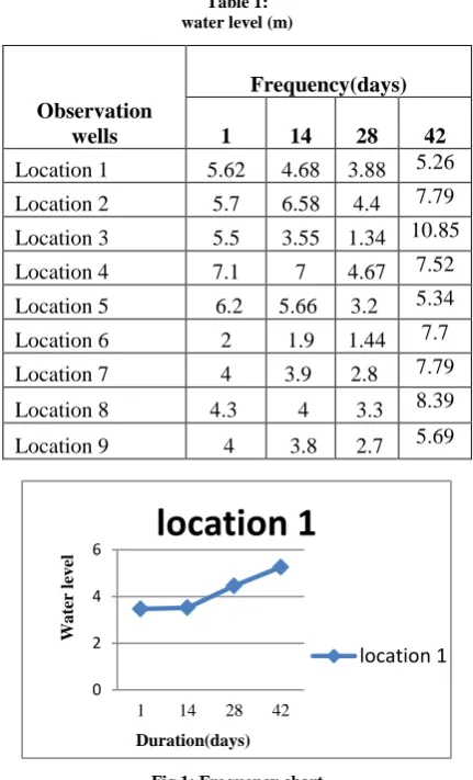
[image:5.595.323.539.138.494.2]

The water level data must be monitored frequently from the selected observation wells. The interval of 14 days is considered in this study. This water level may decrease or increase based on availability, recharge and discharge capacity of the observation wells. The discharge rates of groundwater can be found by field investigation or used from the secondary data which is available. The collected primary data are used for the preprocessing and and processing of visual MODFLOW and Geo-graphical Information System (GIS)

Table 1: water level (m)

Observation wells

Frequency(days)

1 14 28 42

Location 1 5.62 4.68 3.88 5.26

Location 2 5.7 6.58 4.4 7.79

Location 3 5.5 3.55 1.34 10.85

Location 4 7.1 7 4.67 7.52

Location 5 6.2 5.66 3.2 5.34

Location 6 2 1.9 1.44 7.7

Location 7 4 3.9 2.8 7.79

Location 8 4.3 4 3.3 8.39

Location 9 4 3.8 2.7 5.69

Fig 1: Frequency chart

5. Modelling:

A numerical model for the solution of groundwater flow is developed in recent days. VisualMODFLOW is a groundwater modeling program software. It can be compiled and remedied according to the practical applications. It is a finite-difference modeling program, which simulates groundwater flow in three dimensions

Geographical Information Systems (GIS) (Burrough, 1976) are capable of storing, manipulating, and displaying geographically referenced information. GIS combines spatial database management, statistical analysis and cartographic modelling capabilities within computer hardware and software configurations. The water-table fluctuation (WTF) method provides an estimate of groundwater recharge by analysis of water-level fluctuations in observation wells. The method is based on the assumption that a rise in water-table elevation measured in shallow wells is caused by the addition of recharge across the water table.

R(tj) = Sy×H(tj) x total area 0

2 4 6

1 14 28 42

W

a

te

r

le

v

el

Duration(days)

location 1

(6)

International Journal of Emerging Technology and Advanced Engineering

225

R(tj) (cm) is recharge occurring between times t0 and tj , Sy is specific yield (dimensionless) and H (tj) is the peak water level rise attributed to the recharge period (cm).

Where Using GIS, complex analysis between layers or maps is possible and hence attempts have been made for ground water potential assessment in various parts of the world.

X. CONCLUSIONS

Methods of quantifying the groundwater are discussed in this paper. The increasing demand on groundwater leads to over-exploitation and these negative effects have attracted great attention around the world. To reduce these negative effects, it is necessary to carry out strict groundwater resources management in over-exploited areas. It can be managed by formulating different models like dynamic game model and developing some control methods. Stimulating models are also carried out for the future effectiveness. Various methods can be carried out to calculate the quantity and the flow of groundwater. Quantity can be calculated by determining its inflow and outflow quantity. The inflow can be calculated by determining the amount of recharge and the location of recharge sites. From the above literature surveys it is clear that using water table fluctuation method can be used for the estimation of the recharge sites and quantity which can be recharged or which has been recharged. The graphical mapping can also be carried out for quantifying the groundwater. Groundwater flow and transport models have been applied to investigate a wide variety of hydrogeologic conditions. Groundwater flow models are used to calculate the rate and direction of movement of groundwater. The primary and secondary data which is collected are used for the calibration and modeling. The most widely used numerical groundwater flow model is Visual MODFLOW which is a modular three-dimensional finite-difference groundwater flow model. These models can be used for the future prediction of the groundwater flow and water demand under different exploitation.

REFERENCES

[1] Ramesh.H and mahesha.A(2011), “ Groundwater Modeling to Simulate Groundwater LEVELS Due to Interlinking of River in Varada River Basin,India” IEEE Journals

[2] Fawen Li , Ping Feng , Wei Zhang and Ting Zhang (2013)” An Integrated Groundwater Management Mode Based on Control Indexes of Groundwater Quantity and Level” , Water Resour Manage, vol 27,pp: 3273-3292

[3] Z. Jamshidzadeh and S.A. Mirbagheri (2010),” Evaluation of groundwater quantity and quality in the Kashan Basin, Central Iran”, Desalination, vol 270,pp: 23-30

[4] Ravikumar, G., Shahidhar, T., Krishnaveni, M. and Karunakaran, K(2005),” GIS Based Ground Water Quantity Assessment Model”, International Journal of Civil and Environmental Engineering, vol 1, no 2,pp: 21-30

[5] A. K. Saraf and P.R.Choudhury (1998),” Integrated Remote Sensing and GIS for Groundwater Exploration and Identification of Artificial Recharge Sites”, International Journal of Remote Sensing”, vol. 19, no. 10, pp: 1825-1841

[6] MAO Xiaomin,SHANG Songhao,LIU Xiang

(2002),”Groundwater Level Predictions Using Artificial Neural Networks”,Isinghua Science and Technology ISSN,vol7, pp:574 – 579, 6 december

[7] Md. Marufur Rahman and A. Q. M. Mahbub (2012),” Groundwater Depletion with Expansion of Irrigation in Barind Tract: A Case Study of Tanore Upazila”, Journal of Water Resource and Protection, vol 4,pp: 567-575

[8] Gabriel .T, Timothy K. Gates,Darrell G. Fontane, John W and Ruben L. Porto (2000),”Integration of Water Quantity and Quality in Strategic River Basin Planning”, Journal of Water Resources Planning and Management, vol 126,pp: 85-97

[9] Katrin Erdlenbruch , Mabel Tidball , Georges Zaccour (2014) ,”

Quantity–quality management of a groundwater resource by a water agency”, Environmental Science and Policy, vol. 4, pp: 201 – 214

[10] Janmaizatulriah Jani (2012),” GIS as a tool for modeling groundwater flow”, IEEE Symposium on Business, Engineering and Industrial Applications, vol 978-1-4577-1634 pp 513-517.

[11] SH.X. Wang, Qian and X.L. Hu(2011),” Regional Groundwater Flow Modeling in Zhangye Basin a of Heihe River Watershed, China ”, IEEE 978-1-61284-340-7, pp 185-188.

[12] Izrar Ahmed and Rashid Umar(2009),” Groundwater Flow Modeling of Yamuna–Krishni Interstream, a Part of Central Ganga Plain Uttar Pradesh” , J. Earth Syst. Science, vol 118, pp 507-523.

[13] Jiajia Wang, Kunlong Yin and Jian Chen (2011),” Research and Realization of the Groundwater Analyze Module Based on MapGIS”, IEEE 78-1-61284-848-8, pp 270-277

[14] Mahesh K. Jat, Deepak Khare and P. K. Garg (2009),” Urbanization and its impact on groundwater: a remote sensing and GIS-based assessment approach”, Environmentalist, vol 29, pp: 17-32

[15] Lasya C.R and M. Inayathulla(2015,march),” Groundwater Flow Analysis Using Visual Modflow”, IOSR Journal of Mechanical and Civil Engineering, vol 12, pp 05-09.

[16] Marios A. Sophocleous (1991),” Combining The Soilwater Balance and Water-Level Fluctuation Methods to Estimate Natural Ground- Water Recharge: Practical Aspects”, Journal of Hydrology, vol 124, pp: 229-241

[17] G. N. Pradeep Kumar and P. Anil Kumar (2014),” Development of Groundwater Flow Model Using Visual MODFLOW”, International Journal of Advanced Research, vol 2, pp: 649-656 [18] Qingchun Yang, Wenxi Lu and Yanna Fang (2011),” International

journal in Advances Engineering” , vol 24,pp: 638-642 [19] Jihong, ZHOU Juan and CHEN Nanxiang (2010),” Groundwater

Table Prediction Based on Improved PSO Algorithm and RBF Neural Network”, International Conference on Artificial Intelligence and Computational Intelligence, IEEE 978-0-7695-4225-6, pp 228-232