Reliability equivalence factors for a series parallel system assuming an exponentiated weibull distribution

Reliability equivalence factors for a series­

parallel system assuming an exponentiated 

weibull distribution

Alghamdi, SM and Percy, DF

Title

Reliability equivalence factors for a series­parallel system assuming an 

exponentiated weibull distribution

Authors

Alghamdi, SM and Percy, DF

Type

Book Section

URL

This version is available at: http://usir.salford.ac.uk/32037/

Published Date

2014

USIR is a digital collection of the research output of the University of Salford. Where copyright 

permits, full text material held in the repository is made freely available online and can be read, 

downloaded and copied for non­commercial private study or research purposes. Please check the 

manuscript for any further copyright restrictions.

Proceedings for 8th

IMA International

Conference on

Modelling in

Industrial

Maintenance and

Reliability (MIMAR)

10 - 12 July 2014, Wadham and St

Catherine’s Colleges, University of

Oxford

Reliability equivalence factors for a series-parallel system assuming an

exponentiated Weibull distribution

S. M. Alghamdi and D. F. Percy

Salford Business School, University of Salford, Manchester, M5 4WT, UK: [email protected], [email protected]

Abstract. In this study, we discuss the reliability equivalence factors of a series-parallel system with n series subsystems connected in parallel where subsystem i has ݉_௜ independent and identically distributed components. We assume that each component has an exponentiated Weibull distribution. We consider improving the reliability of the system by (a) a reduction method and (b) several duplication methods: (i) hot duplication; (ii) cold duplication with perfect switch; (iii) cold duplication with imperfect switch. We compute two types of reliability equivalence factors: survival equivalence factors (SREF) and mean equivalence factors (MREF). We illustrate the results obtained with an application example.

1. Introduction

The concept of reliability equivalence factors was introduced by Rade in 1989 and published by him in Rade (1993a,b). He applied this concept to simple systems that consist of one component or two components connected in series or parallel. Later, Sarhan (2000, 2005) and Sarhan et al. (2008) applied this concept to more general systems. Most of the designs considered have components with exponential lifetime distributions although some studies applied this concept to other lifetime distributions, such as the Weibull distribution (El-Damcese, 2009) and gamma distribution (Xia and Zhang, 2007).

There are two main methods for improving a system’s design. The first method is reduction, which

involves improving the reliability of the system by reducing the failure rate by a factor ߩ for some of the system components, where ߩ א ሺͲǡͳሻ. This can be achieved by replacing standard components with more expensive, higher quality components. The second method for improving a system’s design is redundancy

duplication, which involves adding extra components in parallel to existing system components. There are three ways to add extra components to the system: hot duplication; cold duplication with perfect switch; cold duplication with imperfect switch. Sometimes, and for many different reasons such as high cost and space limitation, it is impossible to improve the reliability of the system by the redundancy duplication method. Reliability equivalence factors refer to the factors by which the failure rates of some of the system’s

components must be reduced in order to reach equality of the system reliability with that of a better system. In this study, we consider a series-parallel system and assume that all the system’s components are independent and follow the exponentiated Weibull distribution with identical parameters (Mudholkar and Srivastava, 1993). Firstly, we compute the reliability function and the mean time to failure (MTTF) of the original system. Secondly, we compute the reliability functions and MTTFs of the systems following improvement according to reduction, hot duplication and cold duplication (perfect and imperfect) methods. Thirdly, we equate the reliability function and the MTTF of the system improved according to the reduction method with the reliability function and the MTTF of the system improved according to each of the duplication methods to determine the reliability equivalence factors. Finally, we illustrate the results obtained with an application example by presenting table and figures.

2. Series-parallel system

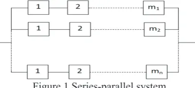
The system we consider here is shown in Figure 1 and consists of n subsystems connected in parallel, where subsystem i consists of ݉_௜components that are connected in series for ݅ ൌ ͳǡʹǡ ǥ ǡ ݊. Such a system is usually referred to as a series-parallel system (El-Damcese, 2009), though some authors refer to it as a parallel-series system.

We assume that the lifetimes of all the system’s components are independent and follow the

exponentiated Weibull distribution with identical parameters (Mudholkar and Srivastava, 1993; Lai, 2014). The exponentiated Weibull distribution generalizes well known lifetime distributions including Weibull with two parameters, Rayleigh and generalized Rayleigh distributions.

Let ݎ_௜௝ሺݐሻ be the reliability function of component ݆ሺ݆ ൌ1ǡ2ǡ ǥ ǡ ݉_௜ሻ _{in subsystem} ݅ሺ݅ ൌ1ǡ2ǡ ǥ ǡ ݊ሻ _and

let ܴ_௜ሺݐሻbe the reliability function of subsystem i . The above assumption implies that ݎ_௜௝ሺݐሻ ൌ ݎሺݐሻ where ݎሺݐሻ ൌ1െ ቀ1െ ݁ିఈ௧ഁቁఏ ₍₁₎

for ݐ ൒ Ͳ, as the lifetimes of components are unaffected by failures of other components. The reliability function of subsystem i then takes the form

ܴ_௜ሺݐሻ ൌ ς ൜1െ ቀ1െ ݁ିఈ௧ഁቁఏൠ ൌ ൜1െ ቀ1െ ݁ିఈ௧ഁቁఏൠ ௠೔

௠೔

௝ୀ1 (2)

for ݐ ൒ Ͳ, so the reliability function of the series-parallel system is

ܴሺݐሻ ൌ1െ ς ሼ௡ 1െ ܴ_௜ሺݐሻሽ

௜ୀ1 ൌ1െ ς ቈ1െ ൜1െ ቀ1െ ݁ିఈ௧

ഁ

ቁఏൠ௠೔቉

௡

௜ୀ1 (3)

for ݐ ൒ Ͳ, and the mean time to failure of the series-parallel system is given by

ܯܶܶܨ ൌ ׬ ܴሺݐሻ݀ݐ ൌ ׬ ቆ1െ ς ቈ1െ ൜1െ ቀ1െ ݁ିఈ௧ഁቁఏൠ ௠೔

቉

௡

௜ୀ1 ቇ ݀ݐ

∞ 0 ∞

0 (4)

3. Designs of improved systems

The two main approaches for improving a system are reduction methods and standby redundancy (duplication) methods. The latter comprise two variations, hot duplication and cold duplication. Furthermore, cold duplication can be performed with perfect switch or imperfect switch. In this section, we derive the reliability function and the mean time to failure for series-parallel systems improved according to the methods identified above.

3.1 Reduction method

As mentioned in the introduction, the reliability of a system can be improved by reducing the failure rate for

some of the system’s components by a factor

ߩ א ሺ

0

ǡ

1

ሻ

components by a factor ߩ, in order to reduce the failure rate (hazard function) for the whole system. This is a logical procedure for the exponentiated Weibull distribution.

Define ܽ_௜ሺ݅ ൌ1ǡ2ǡ ǥ ǡ ݊ሻ _{to be the number of components in subsystem i whose failure rate is reduced, so}

ܽ௜ א ሼ0ǡ1ǡ ǥ ǡ ݉௜ሽand the cardinality of the set of improved components is ȁܣȁ ൌ σ ܽ௡௜ୀ1 ௜. By comparison

with Equation (2), we see that the reliability function ܴ_௜ሺ஺ሻሺݐሻof subsystem i is then given by ܴ_௜ሺ஺ሻሺݐሻ ൌ ൜1െ ቀ1െ ݁ିఈ௧ഁቁఏൠ

௔೔

൜1െ ቀ1െ ݁ିఈ௧ഁቁఏൠ ௠೔ି௔೔

(5)

for ݐ ൒0_{from Equation (1) and by comparison with Equation (3), since the components are connected in}

series. Then the reliability function of the system takes the form ܴሺ஺ሻሺݐሻ ൌ1െ ς ቈ1െ ൜1െ ቀ1െ ݁ିఘఈ௧ഁቁఏൠ

௔೔

൜1െ ቀ1െ ݁ିఈ௧ഁቁఏൠ ௠೔ି௔೔

቉

௡

௜ୀ1 (6)

since the subsystems are connected in parallel. We can then compute the mean time to failure of this series-parallel system as

ܯܶܶܨሺ஺ሻൌ ׬ ቆ1െ ς ቈ1െ ൜1െ ቀ1െ ݁ିఘఈ௧ഁቁఏൠ ௔೔

൜1െ ቀ1െ ݁ିఈ௧ഁቁఏൠ ௠೔ି௔೔

቉

௡

௜ୀ1 ቇ ݀ݐ

∞

0 (7)

3.2 Duplication methods

Now we obtain the corresponding reliability measures of the system when it is improved by duplication. We derive the reliability function and the mean time to failure of the series-parallel system improved according to the hot duplication method and the cold duplication methods with perfect and imperfect switches.

This means that some of the system components are duplicated in parallel by similar components. We assume that in the hot duplication method each component of the set B is augmented by introducing a new but identical component in the same subsystem.

Let ܾ_௜ሺ݅ ൌ1ǡ2ǡ ǥ ǡ ݊ሻ _{be the number of components in subsystem i whose reliability is improved}

according to the hot duplication method, so ܾ_௜ א ሼ0ǡ1ǡ ǥ ǡ ݉_௜ሽ _and ȁܤȁ ൌ σ ܾ௡ _௜

௜ୀ1 . The reliability function ܴ_௜ሺ஻ሻሺݐሻ of subsystem i is given by

ܴ_௜ሺ஻ሻሺݐሻ ൌ ൜1െ ቀ1െ ݁ିఈ௧ഁቁ

2ఏ

ൠ௕೔൜1െ ቀ1െ ݁ିఈ௧ഁቁఏൠ ௠೔ି௕೔

(8) since the components are connected in series. Then the reliability function of the system takes the form ܴሺ஻ሻሺݐሻ ൌ1െ ς ቈ1െ ൜1െ ቀ1െ ݁ିఈ௧ഁቁ

2ఏ

ൠ௕೔൜1െ ቀ1െ ݁ିఈ௧ഁቁఏൠ ௠೔ି௕೔

቉

௡

௜ୀ1 (9)

for ݐ ൒ Ͳ, and the mean time to failure of this series-parallel can then computed as

ܯܶܶܨሺ஻ሻ ൌ ׬ ቆ1െ ς ቈ1െ ൜1െ ቀ1െ ݁ିఈ௧ഁቁ

2ఏ

ൠ௕೔൜1െ ቀ1െ ݁ିఈ௧ഁቁఏൠ ௠೔ି௕೔

቉

௡

௜ୀ1 ቇ ݀ݐ

∞

0 (10)

3.2.2 Cold duplication method with perfect switch

This approach to improving system reliability means that a similar component is connected with an original component in such a way that it is activated immediately upon failure of the original component. For this aspect of our analysis, the cold duplication method assumes that each component of a set C is improved by introducing a new but identical component with a perfect switch.

Let ܿ_௜ሺ݅ ൌ1ǡ2ǡ ǥ ǡ ݊ሻ _{be the number of components in subsystem i, whose reliability is improved}

according to the cold duplication method with perfect switch, so ܿ_௜ א ሼ0ǡ1ǡ ǥ ǡ ݉_௜ሽ _and ȁܥȁ ൌ σ ܿ௡ _௜Ǥ ௜ୀ1

Let ݏ1ሺݐሻ be the reliability function of each component whose reliability is improved according to cold duplication with perfect switch. Regarding a definition of cold duplication with perfect switch, we can describe this improvement as a renewal process with only one renewal (Gamiz et al., 2011). Using the convolution technique, the reliability function of each component whose reliability is improved according to cold duplication with perfect switch can be derived as:

ݏ1ሺݐሻ ൌ1െ ׬

ିௗ௥ሺ௫ሻ

ௗ௫ ሾ1െ ݎሺݐ െ ݔሻሿ݀ݔ ௧

0 (11) where r(t) is the reliability function for the exponentiated Weibull lifetime distribution presented in

Equation (1). By comparison with Equation (2), we see that the reliability function ܴ_௜ሺ஼ሻሺݐሻ of subsystem i is given by

ܴ_௜ሺ஼ሻሺݐሻ ൌ ሼݏ1ሺݐሻሽ௖೔൜1െ ቀ1െ ݁ିఈ௧

ഁ

ቁఏൠ௠೔ି௖೔ (12)

for ݐ ൒ Ͳ, from Equation (1), since the components are connected in series. Then the reliability function of the system takes the form

ܴ_௜ሺ஼ሻሺݐሻ ൌ1െ ς ቈ1െ ሼݏ₁ሺݐሻሽ௖೔൜1െ ቀ1െ ݁ିఈ௧ഁቁఏൠ ௠೔ି௖೔

቉

௡

௜ୀ1 (13) since the subsystems are connected in parallel. We can then compute the mean time to failure of this series-parallel system as

ܯܶܶܨሺ஼ሻൌ ׬ ቆ1െ ς ቈ1െ ሼݏ₁ሺݐሻሽ௖೔൜1െ ቀ1െ ݁ିఈ௧ഁቁఏൠ ௠೔ି௖೔

቉

௡

௜ୀ1 ቇ ݀ݐ

∞

0 (14)

3.2.3 Cold duplication method with imperfect switch

This approach to improving system reliability means that a similar component is connected with an original component by a cold standby via a random switch having a constant failure rate. For this aspect of our analysis, the cold duplication method assumes that each component of a set D is improved by introducing a new but identical component with an imperfect switch.

Let ݀_௜ሺ݅ ൌ1ǡ2ǡ ǥ ǡ ݊ሻ _{be the number of components in subsystem i, whose reliability is improved}

according to the cold duplication method with imperfect switch, so ݀_௜ א ሼ0ǡ1ǡ ǥ ǡ ݉_௜ሽ _and ȁܦȁ ൌ σ ݀௡ _௜Ǥ ௜ୀ1

perfect switch but with the extra condition that the switch is not 100% reliable (Billinton and Allan, 1992), we have

ݏ2ሺݐሻ ൌ1െ ׬

ିௗ௥ሺ௫ሻ

ௗ௫ ሾ1െ ݎሺݐ െ ݔሻݏ3ሺݔሻሿ݀ݔ

௧

0 (15)

where ݎሺ ሻ was defined previously for cold duplication with perfect switch, and ݏ3ሺݐሻ is the reliability function for the imperfect switch. The imperfect switch is chosen to have a constant failure rate ߣ, which means it has an exponential lifetime distribution with parameter ߣ

ݏ3ሺݔሻ ൌ ݁ିఒ௫ (16) The reliability function ܴ_௜ሺ஽ሻሺݐሻ of subsystem i, the reliability function of the series-parallel system ܴሺ஽ሻ_{ሺݐሻ, and the mean time to failure of this system ܯܶܶܨ}ሺ஽ሻ _{can be obtained by comparison with}

Equations (12,13,14).

4. Reliability equivalence factors

According to El-Damcese (2009), “A reliability equivalence factor is a factor by which a characteristic of

components of a system design has to be multiplied in order to reach equality of a characteristic of this design and a different design regarded as a standard”.

We compute two types of reliability equivalence measures. The first type involves survival reliability equivalence factors (SREFs) and these are determined from the reliability or survival function. The second type involves mean reliability equivalence factors (MREFs) and these are determined from the mean time to failure.

4.1 Survival reliability equivalence factors

The idea of SREFs is to assess what degrees of intervention are required to establish equivalence between the reliability functions of a system whose reliability is improved according to one of the duplication methods and a system whose reliability is improved according to the reduction method. That is, to derive the SREFs, we have to solve the following set of equations

ܴሺ஺ሻሺݐሻ ൌ ܴሺுሻሺݐሻ ൌ ߱ǡܪ ൌ ܤǡ ܥǡ ܦ (17) 4.2 Mean reliability equivalence factors

The idea of MREFs is to assess what degrees of intervention are required to establish equivalence between the mean time to failure of a system whose reliability is improved according to one of the duplication methods and a system whose reliability is improved according to the reduction method. That is, to derive the MREFs, we have to solve the following set of equations

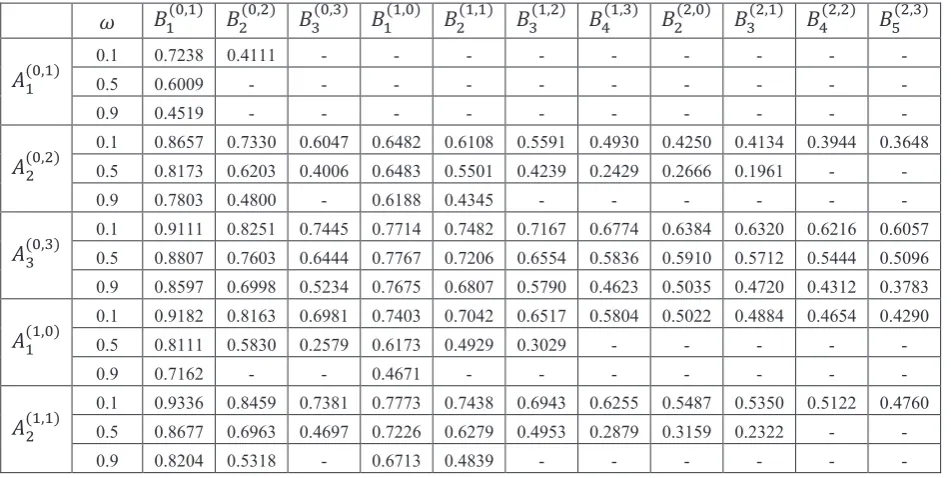
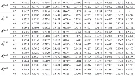
ܯܶܶܨሺ஺ሻሺݐሻ ൌ ܯܶܶܨሺுሻሺݐሻ ൌ ߱ǡܪ ൌ ܤǡ ܥǡ ܦ (18) Table 1 Hot survival reliability equivalence factors

߱ ܤ_ଵሺ଴ǡଵሻ ܤ_ଶሺ଴ǡଶሻ ܤ_ଷሺ଴ǡଷሻ ܤ_ଵሺଵǡ଴ሻ ܤ_ଶሺଵǡଵሻ ܤ_ଷሺଵǡଶሻ ܤ_ସሺଵǡଷሻ ܤ_ଶሺଶǡ଴ሻ ܤ_ଷሺଶǡଵሻ ܤ_ସሺଶǡଶሻ ܤ_ହሺଶǡଷሻ

ܣ_ଵሺ଴ǡଵሻ

0.1 0.7238 0.4111 - - - -

0.5 0.6009 - - - -

0.9 0.4519 - - - -

ܣሺ଴ǡଶሻ_ଶ

0.1 0.8657 0.7330 0.6047 0.6482 0.6108 0.5591 0.4930 0.4250 0.4134 0.3944 0.3648 0.5 0.8173 0.6203 0.4006 0.6483 0.5501 0.4239 0.2429 0.2666 0.1961 - -

0.9 0.7803 0.4800 - 0.6188 0.4345 - - - -

ܣሺ଴ǡଷሻ_ଷ

0.1 0.9111 0.8251 0.7445 0.7714 0.7482 0.7167 0.6774 0.6384 0.6320 0.6216 0.6057

0.5 0.8807 0.7603 0.6444 0.7767 0.7206 0.6554 0.5836 0.5910 0.5712 0.5444 0.5096 0.9 0.8597 0.6998 0.5234 0.7675 0.6807 0.5790 0.4623 0.5035 0.4720 0.4312 0.3783

ܣ_ଵሺଵǡ଴ሻ

0.1 0.9182 0.8163 0.6981 0.7403 0.7042 0.6517 0.5804 0.5022 0.4884 0.4654 0.4290

0.5 0.8111 0.5830 0.2579 0.6173 0.4929 0.3029 - - - - -

0.9 0.7162 - - 0.4671 - - - -

ܣሺଵǡଵሻ_ଶ

0.1 0.9336 0.8459 0.7381 0.7773 0.7438 0.6943 0.6255 0.5487 0.5350 0.5122 0.4760

0.5 0.8677 0.6963 0.4697 0.7226 0.6279 0.4953 0.2879 0.3159 0.2322 - -

ܣሺଵǡଶሻ_ଷ

0.1 0.9451 0.8730 0.7848 0.8167 0.7894 0.7491 0.6937 0.6327 0.6219 0.6041 0.5762

0.5 0.9013 0.7773 0.6259 0.7959 0.7295 0.6419 0.5283 0.5410 0.5062 0.4552 0.3808

0.9 0.8732 0.6922 0.3914 0.7749 0.6667 0.5078 0.1574 0.3384 0.2208 - -

ܣሺଵǡଷሻ_ସ

0.1 0.9537 0.8945 0.8248 0.8497 0.8284 0.7976 0.7565 0.7129 0.7055 0.6932 0.6744 0.5 0.9222 0.8286 0.7224 0.8423 0.7940 0.7331 0.6600 0.6679 0.6467 0.6173 0.5780

0.9 0.9030 0.7753 0.6084 0.8318 0.7587 0.6643 0.5433 0.5876 0.5539 0.5086 0.4473

ܣሺଶǡ଴ሻ_ଶ

0.1 0.9594 0.9095 0.8532 0.8731 0.8560 0.8315 0.7991 0.7647 0.7588 0.7491 0.7341

0.5 0.9085 0.8090 0.7070 0.8230 0.7747 0.7169 0.6511 0.6580 0.6395 0.6141 0.5807 0.9 0.8697 0.7185 0.5488 0.7828 0.7003 0.6026 0.4894 0.5295 0.4988 0.4590 0.4071

ܣሺଶǡଵሻ_ଷ

0.1 0.9634 0.9167 0.8617 0.8813 0.8645 0.8401 0.8073 0.7722 0.7661 0.7562 0.7407

0.5 0.9235 0.8332 0.7333 0.8463 0.8004 0.7433 0.6757 0.6829 0.6635 0.6366 0.6009

0.9 0.8954 0.7612 0.5929 0.8201 0.7441 0.6483 0.5297 0.5726 0.5399 0.4966 0.4390

ܣሺଶǡଶሻ_ସ

0.1 0.9669 0.9239 0.8720 0.8907 0.8747 0.8512 0.8193 0.7846 0.7785 0.7685 0.7530

0.5 0.9352 0.8563 0.7649 0.8679 0.8268 0.7742 0.7099 0.7169 0.6980 0.6715 0.6355

0.9 0.9144 0.8008 0.6489 0.8513 0.7859 0.7004 0.5879 0.6296 0.5979 0.5548 0.4952

ܣሺଶǡଷሻ_ହ

0.1 0.9700 0.9308 0.8831 0.9004 0.8856 0.8640 0.8344 0.8020 0.7963 0.7869 0.7723

0.5 0.9443 0.8762 0.7968 0.8863 0.8507 0.8050 0.7486 0.7548 0.7381 0.7147 0.6826

0.9 0.9283 0.8336 0.7071 0.8756 0.8211 0.7500 0.6559 0.6909 0.6644 0.6280 0.5771 5. Numerical results and analysis

Suppose that we have a series-parallel system consisting of two subsystems connected in parallel. The first subsystem has two components connected in series and the second subsystem has three components connected in series. This means that ݊ ൌ ʹǡ ݉_ଵൌ ʹǡ ݉_ଶൌ ͵ and the total number of components is ݉ ൌ ͷ.

All of the system’s components are assumed to be independent and identically distributed, with lifetimes that

behave according to an exponentiated Weibull distribution with parameters ߙ ൌ ͳǡ ߚ ൌ ʹǡ ߠ ൌ ͵. We define: · ܣሺ௜ǡ௝ሻ_௞ ǡ ݅ ൌ Ͳǡͳǡʹǡ ݆ ൌ Ͳǡͳǡʹǡ͵ƒ†݇ ൌ ݅ ൅ ݆ to represent a reduction method that requires us to reduce

the failure rate of i components from the first subsystem and j from the second subsystem.

· ܤ_௞ሺ௜ǡ௝ሻǡ ݅ ൌ Ͳǡͳǡʹǡ ݆ ൌ Ͳǡͳǡʹǡ͵ƒ†݇ ൌ ݅ ൅ ݆ to represent hot duplication methods when i components are added to the first subsystem and j to the second subsystem.

· Same thing for ܥ_௞ሺ௜ǡ௝ሻ and ܦ_௞ሺ௜ǡ௝ሻ but for cold duplication with perfect and imperfect switch.

For this scenario, in Tables 1 the SREFs for hot duplication are calculated using Matlab according to the above formulae where ߱ is chosen to be 0.1, 0.5, 0.9. For more discussions based on the results presented in Table 1 and Figures 2 and 3, it may be observed that:

· Reducing the failure rate of one component in the second subsystem (which we denote as ܣ_ଵሺ଴ǡଵሻ) by setting ߩ ൌ ͲǤ͹ʹ͵ͺ improves the reliability of the system like adding one component to the second subsystem (which we denote as ܤ_ଵሺ଴ǡଵሻ) according to a hot duplication method where the reliability function of the system is chosen to be ߱ ൌ ͲǤͳ.

· Missing values of the SREFs mean that it is not possible to reduce the failure rate for the set A of components in order to improve the system reliability to be equivalent with the system reliability that can be obtained by improving the set B of components according to hot duplication methods. We can note the same thing clearly in Figure 3.

· Figure 2 explains the improvement strategies to calculate the SREFs. · MTTFs increase with decreasing ߩfor all possible sets A, see Figure 3.

References

Billinton R, Allan R, (1992). Reliability evaluation of engineering systems-concepts and techniques. Plenum Press, New York.

El-Damcese M, (2009). Reliability equivalence factors of a series-parallel system in Weibull distribution. International Mathematical Forum, 4(19):941–951.

Gamiz M, Kulasekera K, Limnios N, Lindqvist B, (2011). Applied nonparametric statistics in reliability. Springer.

Lai CD, (2014). Generalized Weibull distributions. Springer.

Mudholkar GS, Srivastava DK, (1993). Exponentiated Weibull family for analyzing bathtub failure-rate data. IEEE Transactions on Reliability, 42(2):299–302.

Rade L, (1993a). Reliability equivalence. Microelectronics Reliability, 33(3):323–325.

Rade L, (1993b). Reliability survival equivalence. Microelectronics Reliability, 33(6):881–894.

Sarhan A, (2000). Reliability equivalence of independent and non-identical components series systems. Reliability Engineering & System Safety, 67(3):293–300.

Sarhan A, (2005). Reliability equivalence factors of a parallel system. Reliability Engineering & System Safety, 87(3):405–411.

Sarhan A, Tadj L, Al-khedhairi A, Mustafa, A, (2008). Equivalence factors of a parallel-series system. Applied Sciences,10:219–230.