Learning, capital embodied technology and aggregate fluctuations

Munich Personal RePEc Archive

Learning, capital-embodied technology

and aggregate fluctuations

Gortz, Christoph and John, Tsoukalas

University of Nottingham, University of Glasgow

June 2011

Learning, Capital-Embodied Technology and

Aggregate Fluctuations

∗

Christoph Görtz

University of Nottingham

John D. Tsoukalas

University of Glasgow

This version: November 2011.

Abstract

Business cycles in the U.S. and G-7 economies are asymmetric: recoveries and expansions tend to be long and gradual and busts tend to be short and sharp. Moreover, this type of asymmetry appears more pronounced in the last two cyclical episodes in the G-7. A large body of work views the last two cyclical U.S. episodes, namely, the“new economy" boom in the late 1990s, and the 2000s housing boom-bust as episodes where over-optimistic be-liefs have played a significant role. These episodes have revived interest in expectations driven business cycles models. However, previous work in this area has not addressed the important asymmetry feature of business cycles. This paper takes a step towards addressing this limitation of expectations driven business cycle models. We propose a generalization of the Greenwood et al. (1988) model with vintage capital and learning about capital em-bodied productivity and show it can deliver fluctuations that are asymmetric as in the U.S. data. Learning, calibrated to match the procyclical forecast precision from the Survey of Professional Forecasters, is crucial for the model’s ability to generate asymmetries. Fore-cast errors generated by the model are shown to: (a) amplify fluctuations, and (b) trigger recessions that mimic in magnitude, duration and depth the typical post WW II U.S. reces-sion.

Keywords:News shocks, expectations, growth asymmetry, Bayesian learning, business cy-cles.

JEL Classification:E2, E3, D83.

1

Introduction

A stylized fact of business cycles is that recoveries and expansions tend to be long and gradual and busts tend to be short and sharp. This is referred to in the literature as growth rate (or steepness) asymmetry (see Sichel (1993)). This feature is observed in many macroeconomic aggregates, including GDP, investment, consumption and hours worked. Skewness is the sum-mary statistic for measuring this type of asymmetry. Table 1 reports the skewness statistic using per capita GDP as a measure of economic activity for post WWII U.S. data; skewness is negative indicating growth asymmetry.1

Another interesting observation from Table 1 is the fact that cycles seem to have become more asymmetric in the last 20 years. The last two episodes display significantly higher (in absolute terms) skewness compared to earlier episodes. Both of these cyclical episodes, namely, the investment boom and bust (1991 Q1 - 2001 Q4) and the housing “bubble" (2001 Q4 - 2009 Q2) are highly asymmetric episodes as can be seen from Table 1. This feature is not uniquely related to the U.S. economy. Business cycles have tended to become more asymmetric in all G-7 countries as can be seen from Table 2. Interestingly, these episodes have been largely linked with shifts in expectations. Both the investment and housing booms in the U.S. have been associated with over-optimistic beliefs about profitability of future technologies for the former and housing capital gains through never ending house price appreciation for the latter (Shiller (2007)). And in both cases the booms ended abruptly. Fixed capital investment declined by 6.5% during the short 2001 recession whereas house prices and housing investment fell by approximately 30% and 50% respectively from their peaks in 2006 to 2008 (see Mian and Sufi (2010)) without an apparent observable negative disturbance.

Partly motivated by the U.S. investment boom in the 1990s and the associated strong link with expectations, a new literature seeking to explain business cycles based on shifts in ex-pectations has emerged (referred to as the “news” literature). A revival of the idea, present in the early writings of Beveridge (1909), Pigou (1926) and Clark (1935), that cycles can occur without any change in fundamentals has been formalized successfully in the real business cy-cle (RBC) model by the work of Beaudry and Portier (2004) (henceforth BP) and Jaimovich and Rebelo (2009) (henceforth JR). In early work, Barro and King (1994) pointed out that changes in beliefs about the future cannot generate empirically recognizable business cycles within the standard real business cycle model. Intuitively, news that future productivity will improve creates a wealth effect where agents finance the consumption of goods and leisure today from lower investment. Not surprisingly BP, JR and other studies have focused almost exclusively on aligning thenews drivenmodel comovement properties with the pattern of

co-1_{More specifically, negative skewness implies negative changes in GDP are more extreme than positive changes}

movements present in the data, whereby consumption, investment and hours worked co-move with economic activity.2

Thus, previous work has not addressed the important asymmetry feature of business cycles. This paper takes a step towards addressing this limitation of expectations driven business cycle (EDBC) models. We show a simple one sector model with capital embodied productivity can generate business cycles from expectations shifts that are asymmetric as in the data. We con-sider capital embodied productivity as the sole driving force in the model given the evidence suggesting it is a major driving factor of U.S. macroeconomic fluctuations (see e.g. Fisher (2006), Justiniano and Primiceri (2008), Justiniano et al. (2010), Justiniano et al. (2011)). The two key assumptions in the model are: (1) the vintage view of capital productivity, whereby each successive vintage has (potentially) different productivity and (2) agents imperfect infor-mation and (procyclical) learning about this productivity. Moreover, the assumption of vintage specific productivity, introduces learning in a natural way into the model—thus it takes time before agents know the true productivity of a specific vintage. Importantly, empirical evidence finds this type of learning to be significant in plants equipped with new capital equipment as reported in Bahk and Gort (1993) and Sakellaris and Wilson (2004). Bahk and Gort (1993) con-clude: ”Industry wide learning appears to beuniquely related to embodied technical change in physical capital.” Essentially the model we propose can be interpreted as a generalization of Greenwood et al. (1988) with the incorporation of Bayesian learning. Agents receive news about the productivity of future capital vintages. However, news can be noisy and agents solve a signal extraction problem in order to decide on optimal investment, utilization, hours worked and output produced and consumed.

A procyclical speed of learning (or procyclical forecast precision) is an essential compo-nent for the model to generate the asymmetry documented above. In the model, forecasts about capital productivity are more precise near the peak of the cycle than near the trough. Thus an unfavorable signal about capital productivity is more informative at the peak of the cycle and leads agents to cut back investment, hours, utilization and output sharply, since agents have a lot of confidence in their forecast of productivity. By contrast, after the trough and the be-ginning of the recovery, forecast precision is low and signals are difficult to disentangle from noise. Agents respond more cautiously and the expansion phase is more gradual. It is important to note that procyclical forecast precision is documented in surveys that publish forecasts for macroeconomic aggregates such as the Survey of Professional Forecasters (SPF) or the Liv-ingston Survey that pool together forecasts from professionals. The assumption that delivers procyclical forecast precision in the model in line with the survey evidence is the procyclical

2

adoption rate of technological innovations as suggested by the evidence in Comin (2009). The higher adoption rate of innovations during booms generates more precise information about the productivity of future vintages of capital. A larger share of innovations adopted during booms, reduces the uncertainty (or increases the confidence in a statistical sense) about future capital productivity. Agents forecasts about future vintages become more precise because more adopted innovations increase the likelihood they will diffuse into new capital equipment and consequently make new vintages more productive.

There are other desirable properties of the model. First, it passes the comovement test that has been the key focus in the news literature and can replicate fairly well the standard business cycle statistics. Investment, hours, and consumption move together with output in response to a positive shift in expectations. It is important to stress comovement is a property of the model that obtainsindependentlyof learning. More specifically, there are three elements in the model that deliver comovement in the main macroeconomic aggregates in response to news. The type of preferences proposed by Greenwood et al. (1988) and recently generalized by JR, variable capacity utilization and the presence of vintage specific productivity. An important difference to the analysis in JR is the absence of investment adjustment costs (IAC). While IAC are necessary in the JR model to obtain a procyclical investment response, in our framework the presence of vintage specific productivity acts to boost investment immediately when agents receive news that productivity will be higher in the future. Intuitively, this vintage capital channel operates by affecting the return on investment on the arrival of news. That is, when agents receive news that capital’s productivity will be higher tomorrow they start investing immediately because the higher return on investment can only be realized if they invest today and build new capital that will embody the improved productivity, otherwise, the return is lost. Thus, in a sense, the vintage capital channel plays the role of IAC to facilitate the rise in investment in response to good news.

simi-lar differences in output, hours worked and utilization rates. Consequently, conditional on the measure of forecast errors we use, the learning mechanism in the model magnifies changes in fundamentals. This amplification is consistent with the analysis in Eusepi and Preston (2011) who show how learning can amplify fluctuations. Noise does not only amplify changes in fun-damentals but can also trigger recessions (when true productivity rises but agents forecast a decline) that would not occur in a perfect information economy. We find that noise triggered recessions can generate declines similar in magnitude to declines driven by un-favorable funda-mentals. Remarkably, noise can explain a large share of the (average) peak to trough decline in macroeconomic aggregates observed during post world war II U.S. downturns. It can account for the entire share in the decline of output and consumption and 57 percent of the decline in investment and hours worked.

rather than total factor productivity. Moreover, while Van Nieuwerburgh and Veldkamp (2006) rely on noise that occurs in the production process, our learning framework is tightly linked to evidence on the procyclical adoption of technologies. In addition, we analyze how noise impacts the equilibrium allocations and its importance in generating recessions.

The remainder of the paper is organized as follows: Section 2 describes the model. Section 3 outlines the calibration and computational details. Section 4 presents results from simulations and section 5 concludes.

Table 1: GDP Asymmetries of U.S. Business Cycles

U.S. Cycles Skewness

trough to trough

1958Q2 - 1961Q1 -0.14 1961Q1 - 1970Q4 -0.26 1970Q4 - 1975Q1 0.18 1975Q1 - 1980Q3 0.23 1980Q3 - 1982Q4 0.25 1982Q4 - 1991Q1 -0.17 1991Q1 - 2001Q4 -0.53 2001Q4 - 2009Q2 -1.30

Full sample: 1958Q2-2009Q2 -0.27

Notes. Business cycles dates are from the NBER. Skewness is computed from log first differences of real GDP per capita. For data sources see Appendix 1.

Table 2: GDP asymmetries of G-7 Business Cycles

Canada France Germany Italy Japan UK

Cycles Skewness Cycles Skewness Cycles Skewness Cycles Skewness Cycles Skewness Cycles Skewness

trough to trough trough to trough trough to trough trough to trough trough to trough trough to trough 82Q4-92Q1 -0.36 67Q2-75Q3 -0.24 75Q3-82Q4 0.62 83Q2-93Q4 0.24 94Q1-99Q3 -0.78 75Q3-81Q2 0.50 92Q1-09Q3 -1.30 75Q3-82Q4 0.05 82Q4-94Q2 -0.64 93Q4-10Q1 -1.96 99Q3-03Q2 0.15 81Q2-92Q1 -0.28

82Q4-94Q4 -0.04 94Q2-03Q3 0.04 03Q2-09Q1 -2.31 92Q1-10Q1 -2.49 94Q4-03Q3 -0.34 03Q3-09Q1 -2.42

03Q3-09Q1 -1.83

82Q4-09Q3 -0.78 67Q2-09Q1 0.48 75Q3-09Q1 -0.85 83Q2-10Q1 -1.29 94Q1-09Q1 -2.22 75Q3-10Q1 -0.48

2

The Model

We develop a model close in spirit to Greenwood et al. (1988) (henceforth GHH) with two important differences. First, in contrast to GHH, we interpret capital embodied technology as vintage specific rather than enhancing the productivity of current investment expenditures. This difference implies that productivity of current investment is unknown until capital is in-stalled and used in production. Second, agents receive imperfect signals about the productivity of future capital vintages and use Bayesian learning to form expectations about this productiv-ity. This concept of learning we implement implies that agents make forecast errors that can in turn give rise to fluctuations that would not otherwise arise had agents possessed perfect information.

2.1

Firms

The economy comprises of a continuum of perfectly competitive identical firms with unit mass. Firms produce output, yt, using a Cobb-Douglas production function with three inputs. The

production function is given by,

yt= (utkt)αh1t−α, 0< α <1 (1)

wherekt denotes the sum of all efficiency units of capital available for production in periodt

and is defined by:

∞

X

s=0

qt−skt,s =kt, (2)

wherekt,s is capital of vintagesthat is available at time t. This formulation assumes that the

aggregate capital stock contains distinct vintages of capital which are associated with different levels of productivity, q. In addition, capital can be utilized at different rates. The utilization rate is denoted byutand hours worked byht.

Denoting investment byit, the vintages of capital evolve according to:

kt+1,s = (

it for s= 0

(1₋d(ut))kt,s−1 for s≥1.

(3)

Using (3), the economy’s capital accumulation constraint can be derived from equation (2) as

kt+1 = [1−d(ut)]kt+qt+1it, k0 >0is given. (4)

that capital in periodt+ 1depends on the capital embodied shockqt+1. Thus, the productivity

of investment is unknown until the capital is actually installed.

One can interpret the expressionqin the capital accumulation equation as the productivity of a new vintage of capital, whereas the productivity of installed capital remains constant, or as the efficiency of the production of investment goods. Both interpretations exist in the literature, but the timing differs. Ifqis interpreted as the efficiency of the production of investment goods, it makes sense to assume that there exists information about the production function of these investment goods at the time of the actual production. In the vintage specific case however,

q is interpreted as the productivity of a new vintage of capital, the productivity of which is unknown in the period when investment occurs. The productivity may be known (or at least can be forecasted more accurately) in the period after the investment has been made, i.e. when the capital is actually installed and used in production.3

Finally, the depreciation rate of capital, d(ut), depends positively on the degree of capital

utilization as follows,

d(ut) = δ+µ(uωt −1), µ >0, ω > 1, 0≤δ≤1.

Sinced(ut)is strictly increasing and convex, more intensive use of capital accelerates

depreci-ation exponentially. In this function,ωmeasures the costliness of varying the capital utilization in terms of capital depreciation and the elasticity of marginal capital utilization equalsω₋1. The steady state depreciation rate is given byδ. The parameterµallows to calibrate utilization and depreciation in the steady state independently from each other, consistent with steady state utilization equal to unity.

Firms in this economy maximize profits period by period, that is max

ht,ut,kt

Πt=yt−rtkutkt−

wtht, by renting capital and labor services at the beginning of the period from households in

perfectly competitive factor markets, subject to the production function (1). The rental rate of capital and the real wage rate are denoted byrk

t andwt, respectively.

2.2

Households

The economy is populated by a unit measure of identical, infinitely lived households. The representative household maximizes the discounted stream of expected utilities over its lifetime

max

ct,kt+1,ht,ut E0

∞

X

t=0

βt_U(c

t, ht, xt), 0< β <1. (5)

3

These interpretations ofqand the associated timing assumptions are widespread in the literature. An exception is Greenwood et al. (1988). They interpretqtas the productivity of the capital in periodt+ 1, which is already

subject to a flow budget constraint,

ct+kt+1 = (1−d(ut))kt+wtht+rktutkt (6)

and the capital accumulation equation, (4).

Households supply labor and capital in perfectly competitive markets and earn a wage rate

wtand a rental raterkt.

The utility function is given by

U(ct, ht, xt) =

(ct−φh

1+γ

t xt))1−σ−1

1₋σ , withγ ≥0, φ > 0, σ ≥1,

where

xt=c χ tx

1−χ

t−1, 0≤χ≤1.

The variable ct denotes consumption and ht denotes hours worked. The parameter γ is the

inverse of the Frisch elasticity of labor supply andσis the intertemporal elasticity of substitu-tion parameter. The specificasubstitu-tion of the utility funcsubstitu-tion follows Jaimovich and Rebelo (2009) and nests two preference classes. Forχ = 0the utility function has the properties of the class proposed by Greenwood et al. (1988) and forχ = 1 one obtains preferences as discussed in King et al. (1988). As long asχ >0the utility is time-non-separable in consumption and hours worked. It further implies stationary hours worked. The household’s optimality conditions will be presented collectively in the social planner’s problem formulation in section 2.7.

2.3

Technology

We now describe the technology that determines capital productivity. Our goal in this section is not to develop a fully endogenized model that determines the productivity of future capital vintages but to use a parsimonious way to make learning about capital embodied productivity interesting in our one sector framework.4 _{We assume that the state of productivity of each} future vintage can take on two values, a high value, denoted byηH _{and a low value denoted by}

ηL_{. We furthermore assume that the future level of productivity is influenced by the number of}

general innovations available for adoption. This assumption can be motivated by the fact that in the aggregate, sectors that produce capital equipment benefit from general innovations that are adopted widely across the economy. One such important innovation has been the advent and

4

widespread use of Information Technology (IT).5 Some empirical evidence for this channel is provided in Basu et al. (2003). They report that both IT producing and IT using industries in the U.S. have experienced significant acceleration of total factor productivity (TFP) growth in the post-1995 period, coinciding with the IT equipment investment boom of the 1990s.6 _We parameterize these considerations in the process below,

qt+1 =ηt+1v_tκt +ǫt+1, with 0< κt<1. (7)

where, vtis the number of new general innovations available for adoption in periodt and

ηt+1 is an ergodic two-state Markov process withηt+1 ∈ {ηL, ηH}. The termǫt+1isi.i.d.with

mean zero and constant varianceσ2

ǫ. This latter term constitutes noise in our model.

The number of new general innovations available for adoption follows the process:

vt= (1−ρ) +ρvt−1+ξt, with v0 = 1, 0< ρ <1,

where ξt is i.i.d. with mean zero and variance σ2ξ. We assume only a fraction, κt, of the

available innovations, vt, are adopted since there may be innovations that will not improve

capital’s productivity. We therefore require thatκt ∈(0,1)and assume that it is given by:

κt=

1

1 +exp_{−(τvt−vt−1 vt−1 )}

, τ > 0. (8)

Comin (2009) suggests that the adoption behavior of general innovations is pro-cyclical over the business cycle. The formulation for κt above is consistent with this consideration. The

productivity of future vintages of capital,qt+1 can thus change either (a), as a result of a state

change, (b), a change in the number (or the rate of adoption) of new innovations and (c), noise. The framework we adopt above is similar in flavor to Comin et al. (2009) who endogenize procyclical technology adoption in a multi-sector model.

2.4

Information and Forecasting

We now turn to describe the information assumptions and the expectation formation mechanism in this economy. Agents enter periodtwith information setI_{t≡ {k}t_{, q}t_{, v}t_{, κ}t_{, x}t−1

, ct−1

, it−1

, ut−1

, ht−1

, yt−1

, wt−1

, rt−1

}, wherezt_{denotes the infinite history of any variablezthat belongs}

to the information set above. The agents in this economy face a simple signal extraction

prob-5_{Some have argued that the advent of IT (the computer revolution) and its incorporation into production has}

slowly pushed the average rate of embodied technological change higher (see Greenwood and Yorukoglu (1997), Helpman and Trajtenberg (1994) among others), especially after 1973.

6_{Of course this acceleration of TFP assumes that the official price indices do not fully reflect quality}

lem. They observe the whole history ofqbut do not observe the state,η, or noise,ǫ, separately. Agents know the distribution of the noise,ǫ, and are aware that the signal,η, follows an ergodic two-state Markov process with states ηL _{and η}H _{and a transition matrix Π. For the agent’s}

investment decision today it is essential to forecast tomorrow’s capital productivity. At the be-ginning of periodtagents—conditional onI_{t—form expectations about productivity in period}

t+ 1using Bayesian updating.

Specifically, agents evaluate the posterior probability ofηtto be in a high state as follows:7

P(ηt =ηH|It) =

Ψ(qt|ηt=ηH,It)P(ηt=ηH)

Ψ(qt|ηt =ηH,It)P(ηt=ηH) + Ψ(qt|ηt=ηL,It)(1−P(ηt =ηH))

. (9)

Here, Ψ(_·) denotes a normal probability density function. The probabilities of a state change are described in the transition matrix

Π =

"

pHH pLH

pHL pLL #

, (10)

where pij denotes the probability that the economy transits from state i to state j. From the

ergodicity of the Markov chain it follows that pij ∈ (0,1) and piH +piL = 1. We further

assume the transition matrix Π to be symmetric in order to ensure that all asymmetry in the resulting dynamics is endogenous. This assumption and the previous equality implies that

pHL =pLH andpHH =pLL.

The product of the posterior probabilities that productivity was in state ηL_{, η}H _{in period t}

as computed in (9) above, with the transition matrix imply a prior belief about the probability ofηto be in a certain state in periodt+ 1:

[P(ηt =ηH|It), P(ηt=ηL|It)]Π = [P(ηt+1 =ηH|It), P(ηt+1 =ηL|It)]. (11)

Finally, this prior belief allows agents to form an expectation for the productivity of capital in periodt+ 1. SinceEtǫt+1 = 0, using (7) the expectation is given by

˜

qt+1 =Etη˜t+1vκ_tt, (12)

with η˜t+1 = [P(ηt+1 =ηH|It), P(ηt+1 =ηL|It)] "

ηH

ηL #

,

wherez˜t+1denotes the forecasted value in periodtfor the realization of any variable,zint+ 1.

7

2.5

Procyclical learning

The key ingredient of the model is learning capital’s productivity. Evidence of learning em-bodied productivity in different vintages of capital is documented in Bahk and Gort (1993) and more recently in Sakellaris and Wilson (2004). Using data from 1973 to 1986 consisting of 2,000 firms from 41 industries, Bahk and Gort (1993) find that a plant’s productivity increases by 15 percent over the first fourteen years of its life due to learning effects.8

The learning mechanism in the model has several different components that are essential to deliver procyclical forecast precision. Here, we explain the role played by each component. Equation (7) implies that the productivity of a new capital vintage is determined by the amount of adopted innovations vκt

t , a signal component, η and a noise component, ǫ. Agents cannot

separately observe the signal and noise components but use the Bayesian updating process de-scribed in (9) – (12) to make forecasts for η and therefore next period’s productivity. These three components play different roles in the learning mechanism. More specifically, the signal,

ηtand noise, ǫt, components create the signal extraction problem for the agent (with constant

learning over the cycle) while vκt

t serves to amplify the signal, ηt. This latter component

in-troduces a varying speed of learning and is the key element that delivers procyclical forecast precision and consequently the asymmetries in the model. In detail it works as follows. From equation (7) (since the amount of adopted innovations (vκt

t ) is multiplied with the signal, η),

an increase in the amount of adopted innovations amplifies the signal relative to the noise and subsequently accelerates the precision of agent’s forecast for productivity. The degree of ac-celeration depends on the stage of the cycle. Given our assumption of procyclical adoption of innovations, at the peak of the cycle the amplification of the signal is strong (due to the rise in

vκt

t ) and hence one obtains a relatively precise forecast for next period’s productivity. At this

stage of the cycle, agent’s forecasts react sharply to a negative signal compared to the reac-tion (to an identical signal) near the trough where precision is low. At the peak of the boom, agents learn much faster and therefore a negative signal can potentially trigger a quick and sharp adjustment of the economy. By contrast, at the beginning of an expansion, following a trough, the degree of amplification is small and forecast precision low.9 These features make the boom phase more gradual than the bust phase. Note from equation (8) the degree of change

8_{The idea here is that the installation of new vintages of capital equipment is often associated with}

comple-mentary investments in training workers as well as implementation of new organization structures or management practices and these take time to become fully productive. This process was coined by Arrow (1962), “learning by doing". These considerations suggest learning about the productivity of future vintages as a natural assumption to incorporate in the model. In the model it also takes time for agents to learn the productivity of a new vintage, although there are no explicit “learning by doing" effects. Agents learn over time and asymptotically know with certainty the true productivity of a specific vintage.

9

Its important to note, in thevκt

t function,κt (described in equation (8)) has to vary in order to deliver the

procyclical variations forecast precision (or equivalently procyclical speed of learning). Hadκtbeen constant for

inκt is controlled byτ which is calibrated (discussed in section 3.1 below) such as to deliver

a procyclical share of adopted innovations, vκt

t , in line with the evidence reported in Comin

(2009).

Procyclical learning and forecast precision from the Survey of Professional

Forecast-ers (SPF).The SPF publishes one to five quarters ahead forecasts for GDP.10_{An analysis of the} forecast errors from this survey suggests they are negatively related with detrended GDP, in-dicative of a procyclical forecast precision. This fact has been documented in previous studies, most notably, Van Nieuwerburgh and Veldkamp (2006).11 A key requirement for generating procyclical forecast precision in the model as in the SPF data is a pro-cyclical signal-to-noise ratio. This requires that the variance of the noise term (ǫt+1) rises at a slower rate than the

vari-ance of the signal, amplified by the amount of adopted innovations (ηt+1vκ t

t ) when productivity

increases. In other words, during a boom, the impact of the noise on next period’s productiv-ity becomes relatively smaller compared to the impact of the signal and vice versa during a recession. The signal-to-noise ratio from (7) equals

var(ηt+1vκ t

t )

var(ǫt+1)

=var(vκt

t )

σ2

η

σ2

ǫ

.

Since both the variance of the Markov processσ2

ηand the noise variance are constant, the

signal-to-noise ratio is pro-cyclical ifvar(vκt

t )increases in a boom and decreases in a recession.12

Our assumptions on learning imply a faster rate of innovation adoption improves the quality of forecasts. While the rate of adoption is exogenous in the model a plausible interpretation of this relationship can be provided based on the idea that observing the actions of others re-leases information. Examples and formalizations of this idea can be found in the information aggregation (or social learning) literature (see for example Caplin and Leahy (1994)). A stan-dard set-up in this literature is the presence of noisy private and public information that affects decisions by agents. Observing actions from other agents can potentially release useful infor-mation on unobserved states of nature. In our context, the observation that the adoption rate of innovations rises in booms, may release information that some agents undertake (or have undertaken) investment to develop new technologies. This can potentially make other agents who observe this adoption to infer with higher precision the arrival of new capital vintages that are expected to be more productive. In this context, adoption can be interpreted as an informa-tive (public) signal (through the process of aggregation of information) conferring a posiinforma-tive information externality, that helps agents make more precise forecasts about the productivity

10_{For a description of the survey see, Croushore (1993).}

11_{A similar finding about procyclical forecast precision from the Livingston survey is reported in Jaimovich and}

Rebelo (2009).

12_{Our calibration procedure ensures thatvar(v}κt

t )is procyclical. The noise variance is restricted to be constant

of capital. By contrast, in recessions, the information flow is scarce because very few agents undertake adoption of new technologies. Consequently, a low adoption rate makes agents more uncertain about the quality of new capital equipment.

2.6

Equilibrium

Equilibrium in the decentralized economy described above is a sequence of quantities and prices that solve: (1) firms’ problem, (2) households’ problem and (3) satisfy market clearing. Market clearing implies the aggregate resource constraint,

yt=ct+it. (13)

2.7

The Social Planner Problem

The decentralized economy has a social planner analog. We work with this formulation. A benevolent social planner maximizes the utility of the representative agent (5), subject to the capital accumulation constraint (4) and the resource constraint (13). The planner’s problem can be formulated in a recursive way. At the beginning of periodt, ηt andǫt are realized but

cannot be observed. However, the social planner observes the productivity of capital installed in periodt,qt. The planner uses the forecasting mechanism described in (9) – (12) to form an

expectation about the productivity of the vintage in periodt+ 1,q˜t+1. Hence, the social planner

enters the period with state variablesst = (kt, xt−1,q˜t+1). The state variables determine the

choice of ht, kt+1 and ut. Since the choice of investment depends on q˜t+1, the value of the

state variable kt+1 can differ from the realized capital stock in periodt+ 1. This depends on

the difference betweenq˜t+1 andqt+1 and hence on forecast precision. Consumption in turn is

determined from the recourse constraint. Formally, the planner solves:

V(kt, xt−1,q˜t+1) = max

ht,ut,kt+1

U(ct, xt−1, ht) +βEt|kt,xt−1,q˜t₊₁[V(kt+1, xt,q˜t+2)]

s.t.kt+1 = (1−d(ut))kt+itqt+1

ct= (utkt)αh1t−α−it

xt=c χ tx

1−χ t−1

withx−1,q1 andk0 given.V denotes the value function.

This yields the first-order conditions:

(ct−φh

1+γ

t xt)−σ−χψtcχ−

1

t x

1−χ

ψt−(ct−φh

1+γ

t xt)−σφh

1+γ

t =βEtψt+1(1−χ)Etcχt+1x

−χ

t . (15)

(ct−φh

1+γ

t xt)−σφ(1 +γ)h γ

txt=λt(1−α)(utkt)αh−tα, (16)

πt

λt

= 1

Etqt+1

, (17)

αuα−1

t k

α th

1−α

t =

πt

λt

µωuω−1

t kt, (18)

πt =βEt n

λt+1αuα_t+1k

α−1

t+1h 1−α

t+1 +πt+1(1−δ−µ(uω_t+1−1))

o

, (19)

where πt is the multiplier on the capital accumulation equation, λt is the multiplier on the

resource constraint, andψtthe multiplier on the equation that defines the auxiliary variablext.

Equations (14) and (15) determine optimal consumption. Equation (16) sets the household’s marginal rate of substitution between consumption and hours worked equal to the real wage and determines labor supply. Note that forχ >0, the intertemporal decision for optimal hours worked depends on the real wage rate as well as on consumption. Equation (17) determines the real price of investment and is given by the ratio of the two multipliers. Equation (18) determines the optimal rate of capital utilization by setting the marginal user cost equal to the marginal benefit of capital services. The marginal user costs of capital on the right hand side of the equation consists of the partial derivative of d(ut)with respect tout, which represents the

marginal cost in terms of increased depreciation of using capital at a higher rate. This cost is scaled by1/Etqt+1, which determines current replacement costs of old capital in terms of new

capital. Finally, equation (19) determines optimal investment.

It is important to note that the planner’s problem described above is based on the assumption that the planner does not take into account the effect of optimal choices on the evolution of beliefs. Thus there is no feedback between actions and beliefs in this economy and learning is passive. This is similar to Van Nieuwerburgh and Veldkamp (2006) but different from Eusepi and Preston (2011) who allow actions to affect beliefs. The possibility of active learning would invalidate the Welfare theorems in the social planning economy and hence there will be no decentralized counterpart to the planner’s equilibrium.13 _{The passive learning is reflected in the} iteration process of the social planner described above: Expectations of capital’s productivity

13_{In an economy with active learning the provision of information is a public good and information externalities}

are formed at the beginning of the period. Based on these expectations and the endogenous state variables (kt, xt−1), optimal actions are chosen. Given these, expectations are updated at

the beginning of the next period. This process is repeated until the expectations coincide with the actual policies.

3

Calibration and computation

3.1

Calibration

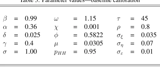
Table 3 reports the parameter values used for calibrating the model. The model is calibrated on a quarterly basis. We assume the depreciation rate of capital,δ = 0.025, quarterly discount factor,β = 0.99 and the capital share of production,α= 0.36. These are all standard values in the literature.

Our calibration of the inverse of the Frisch labor supply elasticity and the parameter which determines the costliness of varying the capital utilization are based on the values used in Jaimovich and Rebelo (2009). Setting the inverse of the Frisch labor supply elasticityγ = 0.4 is a value widely used in the literature implying an intertemporal elasticity of substitution for labor supply of approximately 2.5. In general there are no widely accepted guidelines in the empirical literature about the magnitude for the parameter which determines the costliness of capital utilization. Settingω= 1.15 implies an elasticity of marginal capital utilization of 0.15. We setσ = 1.0 corresponding to logarithmic utility. The parameter that determines the wealth effect on labor supply, χ is set equal to 0.001, (almost) corresponding to GHH preferences, following recent econometric estimates reported in Schmitt-Grohe and Uribe (2008). Finally,

φandµare free parameters and we calibrate these to guarantee that capital utilization is equal to unity and hours worked are equal to one third of the total time endowment in the steady state.14

The following parameters are specific to the learning and the productivity process. In or-der to compute the probability of a state change in productivity we first re-write the ergodic two-state Markov chain as an AR(1) process. Since the transition matrix is symmetric the au-toregressive parameter is given by(2pHH−1). The relative price of investment (i.e. the price

of investment relative to consumption goods) should provide a good empirical measure of the quality improvements embodied in new capital. Hence we use this relative price in order to calibrate the parameters of the productivity process. Specifically, we use the (detrended) mea-sure of relative price of investment constructed by Fisher (2006) which has an autocorrelation of 0.99. There are other estimates (e.g. Greenwood et al. (2000) using a different relative price series) indicating a first-order serial correlation equal to 0.64. We give more weight to Fisher’s

measure and setpHH = (0.9 + 1)/2 = 0.95. It then follows from the structure of the transition

matrix that the probability of a state change equals 0.05.

The parameter τ in the equation that describes κt (equation 8) governs the impact of the

growth rate of general innovations on their adoption rate. While the empirical literature pro-vides indications about the qualitative changes (see Comin (2009)) in the adoption behavior of general innovations over the business cycle, it is silent about the quantitative changes. The role played by τ is to control the amplification of the signal (η) over the business cycle, enabling agents to learn faster during booms but slower during recessions. Calibratingτ= 45 guarantees that the degree of amplification varies continuously from the trough to the peak and thus con-trols the precision of information over the cycle. Specifically forτ _∈ (40,50) the distribution ofκtapproximates a uniform distribution which guarantees thatκtvisits all values in the (0,1)

domain equally during the simulation. By contrast with a high or low value ofτ outside the bounds specified above, the degree of amplification either switches instantly from very low to very high (high values forτ) and vice versa—and stays there for some time— or is almost con-stant over the business cycle (low values forτ). Both cases generate a speed of learning that is mostly constant over the business cycle and imply time series properties of forecast errors from the model inconsistent with the SPF data. Only τ _∈ (40,50), in combination with the cali-bration of volatilities described below, guarantees a procyclical adoption rate and consequently procyclical forecast precision as in the data.

The next objective is to calibrate the standard deviations of the three processes, namely,

ση, σǫ, σε, and the autocorrelation parameter of the adoption process, ρ. Ideally we want to

strike a balance between the size of the noise variance and the variance of the signal such that learning about capital productivity is difficult. The relation between these variances implies a certain signal precision since it determines the difficulty to learn: the noise variance must be high enough to make a boom look like a recession. If it is very low, learning is trivial. However, if the noise variance is very high, estimates about the current state ofηwill be quite inaccurate and this makes learning almost impossible. Estimates for the signal precision of investment-specific technological change are not available due to a lack of forecast data for this variable. We calibrate ση, σǫ, σε andρ in order to match as close as possible three moments from the

SPF: forecast precision (mean absolute forecast error), standard deviation and serial correlation of forecast errors for GDP. This choice guarantees the average “difficulty" of learning in the model is similar to that observed in the SPF.15

The calibration above implies a standard deviation for the noise,σǫ= 0.01. As we compare

percentage deviations in the model the absolute values ofηH _andηL_{are not relevant. However,}

the distance is important since it has an impact on the volatility of the Markov chain. Assigning

15

Table 3: Parameter values—baseline calibration

β = 0.99 ω = 1.15 τ = 45

α = 0.36 χ = 0.001 ρ = 0.8

δ = 0.025 φ = 0.5822 σξ = 0.035

γ = 0.4 µ = 0.0305 ση = 0.07

σ = 1.00 pHH = 0.95 σε = 0.01

the values [0.93, 1.07] toηL_andηH _{implies a standard deviationσ}

η = 0.07. Finally, this

calibra-tion procedure impliesσξ= 0.035 andρ= 0.8.16 The calibration of these parameters guarantees

that the model generates procyclical rate of adoption consistent with Comin (2009).17

3.2

Computational details

The model is solved using value function iteration. We use the policy functions to simulate the model 500 times over 255 periods. The first 50 periods of each simulation are discarded to avoid influences due to the choice of the starting values. Statistics are calculated over the remaining 205 periods corresponding to the sample size (1958 Q2 to 2009 Q2). Second mo-ments are calculated from HP filtered series. Since the model is calibrated on a quarterly basis the smoothing parameter is 1600. Skewness is calculated from first-differenced series.

4

Results

Our first task is to check the model’s ability to generate comovement as stressed by the news literature and highlight the channel that delivers it. In section 4.2 we evaluate the model’s ability to account for the asymmetry of cycles documented in the introduction. Business cycle asymmetry is measured by the skewness of macroeconomic aggregates. The more gradual the boom and the sharper the recession, the more negative is the skewness measure. We also inves-tigate whether the model can match a standard set of business cycle statistics. We then evaluate the effects of learning and focus on, (a) the effects of forecast errors and (b) characteristics of recessions. We are particularly interested in the effects of noise on fluctuations. To do this we compare the outcomes of a model which allows agents to learn over the business cycle with the outcomes of a model without learning (i.e. perfect information case).

16_{We also run simulations of the model withρ= 0.9 orρ= 0.7without any material change in our results.} 17_{In the simulations of the model with the learning mechanism, the correlation between output and the number}

4.1

A simple model without learning: how comovement obtains

In this section we briefly analyze the model’s ability to generate comovement in response to a shift in expectations. This exercise shows that the vintage capital interpretation of productivity is crucial, but that the learning mechanism does not play any role for the model’s ability to generate comovement. For this purpose we analyze a simple version of the model where agents possess perfect information and there is no learning.18 _{Figure 1 presents impulse response} functions (IRFs) from this model. The responses are plotted for one period ahead news shock, i.e. agents receive a perfect signal today there will be a rise in productivity from next period onwards. Figure 1 shows that investment, hours worked, utilization, consumption and output immediately rise in response to good news.

For comparison purposes, the responses from a model with the conventional interpreta-tion of embodied productivity are also presented (model without vintage capital and without learning).19 _{In this case, investment moves countercyclically so this version does not deliver} co-movement. This is not surprising given the absence of investment adjustment costs (IAC) from both models.20 _{As JR demonstrate, IAC is an essential element in a one sector RBC model to} obtain comovement. In the absence of costs in changing the flow of investment, agents can wait until the actual realization of the shock to start investing. But in the vintage capital model IAC are not necessary. The vintage capital specification allows for a channel that affects the return on investment. That is, when agents receive a signal that capital’s productivity will be higher tomorrow they start investing immediately because the higher return on investing can only be realized if they invest today and build new capital that will embody the improved productivity, otherwise, the return is lost. The key difference that makes the vintage capital channel impor-tant is the timing of capital embodiment in the capital accumulation equation, as in equation (4) (i.e. kt+1= [1−d(ut)]kt+qt+1it), which differs from the conventional interpretation only

in the timing of embodiment (i.e.kt+1 = [1−d(ut)]kt+qtit).

4.2

Asymmetries and business cycle statistics

In this section we evaluate the ability of the model to match business cycle statistics computed from U.S. data. We focus on the growth asymmetry, relative volatilities, serial correlations and co-movement. We compute second moments from HP filtered series. We evaluate asymmetry by computing a variable’s skewness from its log first difference. If negative changes are larger

18_{We log-linearize the model’s equilibrium conditions as given in equations (14) – (19) abstracting from}

learn-ing and solve the model with DYNARE.

19_{Since we abstract from learning and to sustain comparability of the IRFs, we use, for both model versions,}

a simple AR(1) process for productivity with an anticipated component. This process has persistence 0.64 and a standard deviation of 0.035 as estimated by Greenwood et al. (2000). All other parameter values are the same as in Table 3.

20

than positive changes then variables will exhibit negative skewness.21 We simulate two versions of the model: a no-learning, perfect information version and the full version which incorporates learning about productivity. In the no-learning version, agents observe the state of ηt at the

beginning of periodt and hence have a perfect signal about productivity (except for thei.i.d.

noise), whereas in the learning version the state ofηtis not revealed.22

Table 4 reports various moments from the data (panel A) and the two versions of the model (panel B and C). Both versions of the model match reasonably well the relative volatilities and correlations with output thereby generating comovement. Moreover, both correctly rank investment to be more volatile than output and consumption to be less volatile than output. However, they under-predict the volatility of hours worked which is more volatile than output in the data.23 They also match reasonably close the serial correlations, although the full model generates slightly lower serial correlations compared with the data. This is a direct consequence of the difference in the serial correlation between the actual,q, and forecasted productivity,q˜. In the learning version, the latter’s serial correlation is markedly lower compared to the true process; for learning to be realistic (i.e. neither impossible nor trivial) the noise shock has to be big enough to make a boom look like a recession. This however implies that agents’ may wrongly infer a state change in capital’s productivity when none has occurred. Thus conceptu-ally, agents’ forecasted productivity is “changing state" more often than true productivity and this imparts a lower autocorrelation in forecasted productivity,q˜.

The main difference between the two versions of the model in Table 4 is with respect to the generated asymmetry. In particular, only the learning version can generate asymmetry in all variables in line with the data (panel C)—the no-learning version fails in this dimension. More precisely the point estimate in the data skewness measure is within two standard deviations of the model’s skewness. This can be seen in the last column of Table 4. In panel B, without procyclical learning, the skewness of output is close to zero, indicating that boom and recession phases are symmetric. Moreover the future productivity of capital, q, has skewness close to zero. Since agents perfectly observe the signal— as the state ofηtis revealed at the beginning of

periodt—their forecast for productivity,q˜, differs fromqonly by the additive noise shock,ǫt+1.

This noise shock on its own is not a source of asymmetry which explains why the skewness of q˜is close to zero and very similar to the one for q. Since there is no other mechanism in

21_{Since the HP filter is a two-sided filter, information from the past as well as the future are used. De-trending}

with this filter implies that agents have information about the future which can have an impact on their decision today. Using a two-sided filter diminishes the filtered values prior to a downturn. This reduces the magnitude of the bust and influences our evaluation of business cycle asymmetry. To avoid this distortionary effect of two-sided filters – such as the commonly used HP or bandpass filter – we calculate the variable’s skewness from the log first-differences.

22

The no learning version of the model differs from Greenwood et al. (1988) only by the fact that productivity of the newly installed capital is subject to the additivei.i.d.shockǫwhich cannot be observed by the agents.

23

the model to make booms longer and more gradual than recessions, all other macroeconomic aggregates exhibit skewness which is close to zero as well. The main reason for the generated growth asymmetry in the learning version is the skewness of agent’s forecast for productivity,

˜

q, which is negative in contrast to the no-learning version. The introduction of agent’s learning over the business cycle is the crucial mechanism to generate growth asymmetries in line with the data. Booms tend to be more gradual than recessions because agent’s speed of learning varies procyclically over the business cycle. Intuitively, during booms forecast precision is high and thus a negative signal about productivity can trigger a quick and sharp adjustment of the economy. By contrast, at the beginning of an expansion, following a trough, forecast precision is low and agents react more cautiously to a positive signal. The asymmetry in agent’s forecast for productivity imparts negative skewness in the remaining macroeconomic aggregates in the learning version as this constitutes the only driving force in the model. This effect is very strong for output, investment, hours worked and capital utilization while it is less so for consumption. These results demonstrate the importance of the learning mechanism to generate the growth asymmetries present in the data. It is interesting to highlight a difference in our results in comparison to Van Nieuwerburgh and Veldkamp (2006) who also analyze asymmetries. A key difference is that in our model asymmetries arise entirely due to procyclical learning. By contrast in Van Nieuwerburgh and Veldkamp (2006) there is built-in asymmetry, i.e. even without learning (see Table 2, page 764) and learning helps to amplify this asymmetry.

4.3

The role of forecast errors: optimism and pessimism

This section provides a more detailed analysis about the functioning of the learning mecha-nism by evaluating the role of forecast errors. Specifically we wish to examine the effects of optimism and pessimism on the cyclical fluctuations of the model. We define an agent as pessimistic (optimistic) when we observe a “large" (to be defined below) negative (positive) forecast error in the simulation. A negative (positive) forecast error implies that agents under-predict (overunder-predict) capital’s productivity relative to the truth.

We examine the distribution of forecast errors obtained from the simulation and choose to examine forecast errors that exceed one standard deviation above or below the average forecast error.24 _{We label those errors as ”large”. This threshold generates forecast errors that occur in} approximately 19% of time in the simulation. We observe large negative forecast errors in 10% of the simulation and large positive forecast errors in 9% of the simulation.25 _{We calculate the}

24

We use the simulation set-up described in section 4.2 and simulate the learning and no-learning economies using an identical sequence of the shocks that determine the productivity of next period’s capital (signal, noise and adoption process shocks).

25

Table 4: Key moments of macroeconomic aggregates

Relative First-order Correlation Skewness std deviation autocorrelation with y

Panel A: U.S. Data

y 1.00 0.85 1 -0.27

i 4.62 0.79 0.90 -0.76 h 1.16 0.91 0.87 -0.74 c 0.80 0.87 0.87 -0.69

Panel B: Model without learning

y 1 0.824 1 0.004

(0.000) (0.042) (0.000) (0.332) i 3.537 0.782 0.948 -0.036 (0.276) (0.047) (0.021) (0.394) h 0.746 0.811 0.992 0.022

(0.009) (0.044) (0.002) (0.331) c 0.387 0.813 0.772 0.026

(0.052) (0.066) (0.047) (0.319) u 1.488 0.818 0.991 0.019

(0.016) (0.044) (0.002) (0.333) q 0.707 0.817 0.944 0.018

(0.018) (0.041) (0.015) (0.318)

˜

q 0.692 0.832 0.970 0.012 (0.015) (0.039) (0.008) (0.332)

Panel C: Model with learning

y 1 0.708 1 -0.171

(0.000) (0.078) (0.000) (0.312) i 3.499 0.670 0.954 -0.170 (0.260) (0.079) (0.017) (0.335) h 0.747 0.695 0.993 -0.157 (0.008) (0.078) (0.002) (0.297) c 0.379 0.742 0.771 -0.043 (0.052) (0.090) (0.043) (0.341) u 1.485 0.701 0.991 -0.194 (0.016) (0.078) (0.002) (0.322) q 0.686 0.812 0.885 0.011

(0.038) (0.045) (0.031) (0.334)

˜

q 0.689 0.710 0.972 -0.189 (0.013) (0.078) (0.006) (0.337)

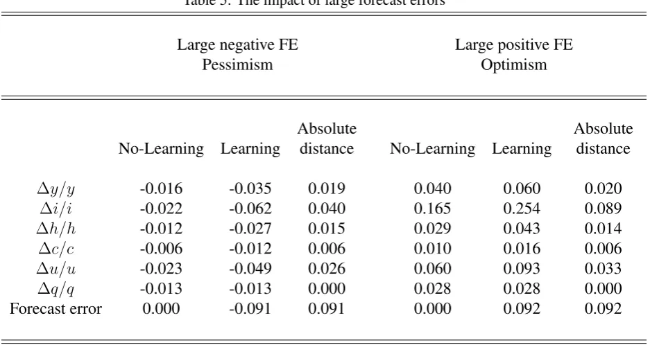
mean growth in variables from the two economies. These results are summarized in Table 5. We draw attention to the following facts from Table 5. First, agents are pessimistic when the true growth rate of productivity is negative and optimistic when the true growth rate of productivity is positive. The presence of noise makes it difficult for agents to accurately pre-dict true productivity when the latter is changing and agents make substantial forecast errors when trying to predict the true process. Second, agents in the no learning economy always forecast capital productivity perfectly—no forecast errors occur in this economy. Changes in fundamentals cause fluctuations in macroeconomic aggregates in both economies but errors in forecasting productivity amplify those fluctuations. The magnitude of amplification is quite substantial. In order to demonstrate this we look at the absolute distance, for each variable, between the learning and no-learning economies—this is reported in the columns labeled ”Ab-solute distance”. This distance quantifies by how much equilibrium allocations differ due to forecast errors, conditional on observing a ”large” forecast error.

The distance in investment growth rates is larger among all variables followed by utiliza-tion, output and hours. The distance in investment growth is equal to 4.0% for negative forecast errors and 8.9% for positive forecast errors. In the learning version, pessimistic agents cut in-vestment on average by 6.2% relative to a modest 2.2% when they possess perfect information. When agents are optimistic they raise investment by 25.4% compared to 16.5% in the perfect information economy. In this case agents over-invest. This is an interesting finding because it has a parallel with the boom in investment rates observed during the IT boom-bust cycle in the 1990s, thought to be driven by excessive optimism about future returns on new investment. When agents are pessimistic, output in the learning economy declines by 3.5% compared to 1.6% in the no learning economy, while in periods of optimism output in the learning economy rises by 6.0% compared to 4.0% in the no learning economy. Similar differences occur in uti-lization rates and hours worked, while the difference in consumption allocations is relatively small.26

4.4

Characteristics of recessions

We also want to examine the nature of recessions in the model economy. We define recessions in the model as periods with at least two quarters of negative output growth. Table 6 reports

26_{Our results on the effects of forecast errors illustrated in this exercise is related to two recent studies.}

Table 5: The impact of large forecast errors

Large negative FE Large positive FE Pessimism Optimism

Absolute Absolute No-Learning Learning distance No-Learning Learning distance

∆y/y -0.016 -0.035 0.019 0.040 0.060 0.020

∆i/i -0.022 -0.062 0.040 0.165 0.254 0.089

∆h/h -0.012 -0.027 0.015 0.029 0.043 0.014

∆c/c -0.006 -0.012 0.006 0.010 0.016 0.006

∆u/u -0.023 -0.049 0.026 0.060 0.093 0.033

∆q/q -0.013 -0.013 0.000 0.028 0.028 0.000 Forecast error 0.000 -0.091 0.091 0.000 0.092 0.092

Notes. Variables included: Output (y), investment (i), hours worked (h), consumption (c), capital utilisation (u), productivity (q) and the forecast error for productivity, computed asEt₋₁qt−qt. The model is simulated 500

times over 255 periods each. The first 50 periods are discarded and the mean growth in variables of the economy with and without learning is calculated over the remaining periods. Forecast errors for productivity are defined to be large when their absolute value exceeds one standard deviation of the average forecast error.

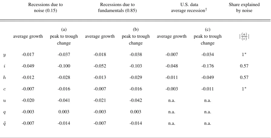
characteristics of recessions from the model and compares them with recessions from the U.S. data. Several findings are worth highlighting. First, the average length of the recession in the model is four quarters, very similar to that in the data (4.25 quarters). Second, recessions in the model can be driven bynoise (with no change in fundamentals) in addition to un-favorable fundamentals. The share of recessions in the model that occur purely due to noise equals 15%. The remaining 85% of recessions are caused by unfavorable fundamentals. The noise triggered episodes coincide with agents mistakenly forecast productivity to be declining when true productivity is actually rising at the onset of the recession. A similar exercise on the nature of recessions is reported in JR. A key difference of our exercise however is that while in their experiment recessions can only arise from bad news about the future, in ours, recessions can also arise due to forecast errors triggered by noise (agents expect productivity to be declining when it is actually improving). Thus our approach can provide a more detailed separation between unfavorable news and noise driven recessions.

the noise triggered compared to 5.2% in the fundamentals triggered recession. Second, the model’s average growth declines match reasonably well the average growth declines in macro-aggregates observed during U.S. recessionary episodes.27 _{For example, the model generates} very similar average growth declines in hours worked, consumption and investment although overpredicts to some extent the output growth decline. We view these findings as a success of the model given it is driven by a single disturbance.

The declines from peak to trough are also similar for the two types of recessions in the model. For example, the decline in output is 3.7% in the noise triggered compared to 3.8% in the fundamentals triggered episode, whereas the peak to trough decline in investment is 10% and 10.3% in the noise and fundamental triggered episodes respectively. Interestingly, the noise driven recession can explain a large fraction of the peak to trough change in macroe-conomic aggregates computed from the data. The last column of Table 6 reports the share of peak to trough decline in the data that can be accounted for by noise in the model. A noise triggered recession can account for all of the decline in output and consumption (arithmeti-cally it accounts for over 100% of the decline in those aggregates) and 57% of the decline in investment and hours worked. This is a remarkable finding given that the model’s exogenous processes were calibrated to match the time series behavior of forecast errors for GDP and not calibrated to match any statistic from Table 6 or statistics from aggregate macroeconomic variables (e.g. volatility and persistence of GDP) that could potentially overweight the model’s ability to match recessions observed in the data.

5

Conclusions

Business cycles in the U.S. and G-7 economies are asymmetric: recoveries and expansions tend to display a long and gradual phase and busts tend to be short and sharp. Moreover, this type of asymmetry appears more pronounced in the last twenty years. Specifically, in the U.S. the last two cyclical episodes have been more asymmetric relative to earlier episodes. Both the investment (in the 1990s) and housing booms and busts (in the 2000s) in the U.S. have been associated with over-optimistic beliefs about profitability of future technology for the former and housing capital gains through never ending house price appreciation for the latter. These episodes have sparked interest in expectation driven business cycles (EDBC), where a sudden shift in agents’ expectations (with no observable change in current fundamentals) can generate aggregate fluctuations as observed in the data. Earlier work in EDBC models have tended to focus in analyzing the model elements that generate comovement (see e.g. Beaudry and

27

Table 6: Recession statistics

Average share of recessions in the model

Recessions due to Recessions due to U.S. data Share explained noise (0.15) fundamentals (0.85) average recession† _{by noise}

(a) (b) (c)

average growth peak to trough average growth peak to trough average growth peak to trough |(₍ac))|

change change change

y -0.017 -0.037 -0.018 -0.038 -0.007 -0.034 1∗

i -0.049 -0.100 -0.052 -0.103 -0.048 -0.176 0.57

h -0.012 -0.028 -0.013 -0.029 -0.011 -0.049 0.57

c -0.007 -0.016 -0.007 -0.016 -0.003 -0.011 1∗

u -0.020 -0.041 -0.021 -0.042 n.a. n.a.

q -0.003 0.003 -0.003 0.003 n.a. n.a.

˜

q -0.007 -0.014 -0.007 -0.014 n.a. n.a.

Notes. Variables included: Output (y), investment (i), hours worked (h), consumption (c), capital utilisation (u), productivity (q) and the forecast for productivity (q˜). Share explained by noise is defined as peak to trough change (due to noise) over peak to trough change in U.S. data.†_{: growth and peak to trough declines computed as the average from all U.S. recessions.}∗_{Shares that exceed one in the Table above are}

set equal to one.

Portier (2004) and Jaimovich and Rebelo (2009) among others) patterns in line with the data comovement properties, whereby consumption, investment and hours worked move together with economic activity.

6

Appendix

Appendix 1: Data

The U.S. data for output is real GDP (GDPC96). Investment is defined as gross private do-mestic investment (GPDIC96) and consumption is real personal consumption expenditures (PCECC96). These series are quarterly, seasonally adjusted and in billions of chained 2005 dol-lars from the U.S. Department of Commerce, Bureau of Economic Analysis (BEA). The series of civilian non-institutional population (CNP16OV), is used to derive per-capita time-series. Hours worked is measured as hours of all persons in the non-farm business sector (HOANBS). The hours and population measures are from the U.S. Department of Labor, Bureau of Labor Statistics.

The forecast error statistics we use for nominal GDP (NGDP) are from the Survey of Pro-fessional Forecasters. This survey pools proPro-fessional forecasters to obtain one to five quarter ahead predictions for different variables and are available from 1968 Q4. We use forecasts from 1968 Q4 to 2009 Q2 to calculate the forecast errors. The forecast error for a given quarter is the log absolute difference between the median of all forecasters predictions for nominal GDP and the final revised value of nominal GDP as it appears today.

Skewness in Tables 1 and 2 are calculated from first differences of real GDP per capita. Real GDP data for all G7 countries (except U.S. and Germany) are from the Organisation for Eco-nomic Development and Cooperation (OECD). Real GDP for Germany is from the Deutsche Bundesbank. All series are quarterly, seasonally adjusted and in chained values. Due to data availability sample size varies by country: Canada (1982Q4 to 2009Q3), France (1967Q2 to 2009Q1), Germany (1975Q3 to 2009Q1), Italy (1983Q2 to 2010Q1), Japan (1994Q1 to 2009Q1), UK (1975Q3 to 2010Q1). The start and end dates correspond to troughs as reported by the Economic Cycle Research committee. Time series for total population are from the World Bank for all G7 countries except the U.S.. We used linear interpolation to transform this data form annual to quarterly frequency.

Appendix 2: Determination of the Parameters

φ

and

µ

from the steady state Euler equation (19):

1 =[β(αuαkα−1

q+ (1₋d(u))]

⇔k=

(

1

β −(1−(δ+µ(u

ω

−1))

1

αuα_q )α1−1

.

We want to calibrate the model in a way that u= 1 when h= 1. Considering the steady state expression for capital utilisation — which can be derived from the first order condition (18) — and using the equation above, one can derive a formulation of steady state utilisation solely depending on parameters:

u=

α µωk

α−1

q

_ω−α1

⇔u=

(

αq µω

1

β −(1−(δ+µ(u

ω

−1)))

1

αuα_q

α−11α−1) 1

ω−α

⇔u=

(

1

β −(1−δ)−µ

1

µ(ω₋1)

)ω1

. (.1)

From this equation one can derive an expression for µas the steady state utilisation is chosen to equal unity:

1 =

"

1

µ(ω₋1)

1

β −(1−δ)−µ

#

1

ω

⇔µ=1

ω

1

β −(1−δ)

.

Note that the choice ofuto equal unity allows to calibrate capital utilisation and depreciation in the steady state independently form each other, asd(u) =δ+µ(uω_{−1) =δ.}

A steady state capital utilisation of unity and a steady state productivity of q = 1 implies that the steady state capital stock can be expressed as:

k =

(

1

βα −

(1₋δ)

α

)α−11

. (.2)

capital utilisation and steady state employment are independent of the value of steady state productivityq. For capital utilisation this is shown in the derivation of equation (.1). The fact that steady state employment is unaffected by the value ofqfollows from the properties of the chosen utility function which guarantee stationary employment.

Appendix 3: Derivation of the Elements of the Bayesian Updating Formula

The Unconditional Probability ofηto be in a Certain State:

The stochastic process for η is designed to be an ergodic two-state Markov process. By def-inition, an ergodic Markov chain has exactly one eigenvalue which equals unity. All other eigenvalues lie inside the unit circle. The eigenvector which is associated with the unit eigen-value is therefore unique and can be interpreted as the vector of unconditional probabilities. For the above described ergodic two-state Markov chain the eigenvector associated with the unit eigenvalue turns out to be

P

(

ηt =ηH

ηt=ηL )

=

1−pLL 2−pH H−pLL

1−pH H 2−pH H−pLL

!

. (.3)

The assumptions of a symmetric transition matrix and an ergodic two-state Markov chain imply thatpHH = pLL. It follows from expression (.3) that the unconditional probability ofη to be

in a high (low) state is 0.5. Thus, the formula for Bayesian updating (9) depends solely on the probability ofqtconditional onηt =ηH andηt =ηL, respectively.

The Normal Probability Density Function:

There is always some uncertainty about the state ofη. Therefore, all inference aboutηtakes the form of statements of probability. Uncertainty is described in terms of the normal probability density function Ψ(_·). Given the mean E(qt|ηt = ηH) and the variance V(qt|ηt = ηH) the

normal probability density for every outcomeqt, given ηt being in a high (low) state, can be

calculated according to

Ψ(qt|ηt=ηH) =

1

V(qt|ηt =ηH)

√

2Πexp −

(qt−E(qt|ηt =ηH))2

2(V(qt|ηt =ηH))2 !

AsEtǫt= 0, the mean and the variance can be derived by using the formulation for productivity

(7):

E(qt|ηt =ηH) =Et[ηHvκ

t−1 t−1 +ǫt]

=ηH_vκt−1 t−1 .

V(qt|ηt =ηH) =Et[(ηHvtκ−t−11 +ǫt)2]−(Et[ηHvκt−t−11 +ǫt])2

=Et[(ηHv κt−1 t−1 )

2

+ 2ηH_vκt−1 t−1 ǫt+ǫ

2

t]−(η H_vκt−1

t−1 ) 2

=σ2

ǫ.