Non Parametric Local Maxima and Minima Finder with Filtering Techniques for Bioprocess

ISSN Online: 2159-4481 ISSN Print: 2159-4465

Non-Parametric Local Maxima and Minima Finder

with Filtering Techniques for Bioprocess

K. K. L. B. Adikaram

_{, M. A. Hussein}

_{, M. Effenberger}

_{, T. Becker}

1_{Group Bio-Process Analysis Technology, Technische Universität München, Freising, Germany}

2_{Bavarian State Research Center for Agriculture, Institute for Agricultural Engineering and Animal Husbandry, Freising, Germany} 3_{Computer Unit, Faculty of Agriculture, University of Ruhuna, Mapalana, Kamburupitiy, Sri Lanka}

4_{Lehrstuhl für Brau-und Getränketechnologie, Technische Universität München, Freising, Germany}

Abstract

Typically extrema filtration techniques are based on non-parametric properties such as magnitude of prominences and the widths at half prominence, which cannot be used with data that possess a dynamic nature. In this work, an extrema identification that is totally independent of derivative-based approaches and independent of quan-titative attributes is introduced. For three consecutive positive terms arranged in a line, the ratio (R) of the sum of the maximum and minimum to the sum of the three terms is always 2/n, where n is the number of terms and 2/3 ≤ R ≤ 1 when n = 3. R > 2/3 implies that one term is away from the other two terms. Applying suitable mod-ifications for the above stated hypothesis, the method was developed and the method is capable of identifying peaks and valleys in any signal. Furthermore, three tech-niques were developed for filtering non-dominating, sharp, gradual, low and high extrema. Especially, all the developed methods are non-parametric and suitable for analyzing processes that have dynamic nature such as biogas data. The methods were evaluated using automatically collected biogas data. Results showed that the extrema identification method was capable of identifying local extrema with 0% error. Fur-thermore, the non-parametric filtering techniques were able to distinguish dominat-ing, flat, sharp, high, and low extrema in the biogas data with high robustness.

Keywords

Extrema Point, First Derivative, Peak Finder, Peaks and Valleys, Maxima and Minima, Second Derivative

1. Introduction

In process control, the method of determining peaks and valleys of a signal, also known as identification of local maxima and minima, is crucial for describing and capturing

How to cite this paper: Adikaram, K.K.L.B., Hussein, M.A., Effenberger, M. and Becker, T. (2016) Non-Parametric Local Maxima and Minima Finder with Filtering Tech-niques for Bioprocess. Journal of Signal and Information Processing, 7, 192-213.

http://dx.doi.org/10.4236/jsip.2016.74018

Received: July 21, 2016 Accepted: October 8, 2016 Published: October 11, 2016

Copyright © 2016 by authors and Scientific Research Publishing Inc. This work is licensed under the Creative Commons Attribution International License (CC BY 4.0).

http://creativecommons.org/licenses/by/4.0/

certain signal properties. Identification of local maxima and minima is particularly useful in signal processing, consequently useful in inline/online process control and op-timization. Thereby, for reliable feature extraction it is necessary to remove redundant maxima and minima in a processed signal. The issue has been extensively investigated in literature [1]-[4], at which different techniques were reported. Magnitude-based methods and gradient-based methods are the most common two of such techniques. In magnitude based methods, the nth _{term of a series is x}

n; xn is considered as a peak

(maximum) when xn−1 < xn > xn+1. In the same time, xn is considered as a valley

(mini-mum) when xn−1 > xn < xn+1. In gradient-based methods, extremum can be located by

considering slope (gradient) of a certain point and acts as the most popular method [1]. When the slope is zero (first derivative is zero) at a certain point, the point can be de-scribed as a peak, valley or a saddle point. However, additional calculations are neces-sary to distinguish whether it is a peak, valley or saddle point. This encounter is solved by analysing the sign of the second derivative at the points of zero slopes [1]. The most popular methods of such are Newton Raphson method [2] and Taylor series-based de-rivatives [3][4] which evaluate the derivatives numerically for a given data set.

Once the extrema points are identified, a filtration step is unavoidable to identify the dominant or relevant extrema. Magnitude of prominences and the widths at half prominence are two properties of signals that are commonly used to filter extrema [5] [6]. Furthermore, baseline correction is another technique used for finding out accurate maxima and minima [7]-[9]. In addition, there are numbers of methods for filtering unnecessary extrema based on template matching or masks [10], such as Kalman filters [11][12] and non-linear filters [13]. Nevertheless, all aforementioned approaches are parametric methods [14], which question their robustness.

One of the main classifications existing in data analysis techniques is whether the method is parametric or non-parametric in its nature [15]. As mentioned above, most popular extrema filtering methods suffer from parametric concerns. Particularly, para-metric methods use domain dependent value as detection criteria such as average, standard deviation, prominences of an extrema, and the widths at half prominence of an extrema. These criteria are based on domain dependent parameters and are there-fore valid only for the considered data model or considered conditions in the domain. Thus, majorly parametric methods’ accuracy inherits the variables’ ranges and the con-ditions of the domain [16]. In reality, data capturing, especially within dynamic sys-tems, such as biogas plants, is produced with various alterations. When the model or data range alters, whilst using parametric methods, it is necessary to recalibrate para-meters or develop new models for monitoring, controlling, and data analysis, which is not of preference at process line.

Non-Parametric Methods

identi-fication and filtration are developed. The proposed technique determines maxima and minima based on the relation of sum of terms in an arithmetic series. The same relation was used as a non-parametric method (MMS: a method based on maximum, minimum, and sum) for finding outliers in linear relation [20] and non-parametric linear fit iden-tification method [21].

In some situations outliers, peaks and valleys are the same, when a sudden extremum (variation) occurs, additionally extrema can be formed due to gradual increment and gradual decrement. The extrema generated in such situations do not behave as outliers and cannot be identified using the aforementioned outlier detection method based on maximum, minimum, and data series sum (MMS) [20]. Furthermore, MMS can only be used for identifying outliers in liner regression and is not suitable for finding outliers in non-linear series [20]. This work focuses on modifying the methods of MMS for lo-cating extrema in non-linear data series.

The proposed extrema identification method does not involve first or second deriva-tive, but rather compares, within a considered window, two ratios in relation with maximum, minimum, middle point, and the sum of data points. Furthermore, three extrema filtration methods were introduced in this work, which are capable of filtering extrema independent of the prominences or width of an extremum. All the methods introduced in this work are developed for harsh conditions involved in dynamic proc-esses, especially biogas process data, thus handling: non-linear datasets and based upon non-parametric methods.

2. Materials and Methods

As mentioned before, the outlier detection method, also by the same authors [20], will be modified to locate extrema in non-linear series. The method is based upon the the-ory of the sum of terms of an arithmetic progression. Having two major relations by means of MMSmax and MMSmin and are expressed in Equation (1) and Equation (2). The

ratio 2/n is used as the detection criteria, where n is the number of terms in the series.

(

) (

)

max max min n min

MMS = a −a S a− ∗n , and (1)

(

) (

)

min max min max n

MMS = a −a a ∗ −n S , (2) where amin is the minimum element of the series, amax is the maximum element of the

series, n is the number of terms in the series, and Sn is the sum of terms in the series.

The complete expression for outlier detection is given by Equation (3). If any series expected to follow y = c form and contains data that do not agree with y = c form then:

(

)

(

)

(

)

(

)

2 ;maximum is the outlier

2 ;

2 ;

2 ;minimum is the outlier n

n

n w

a a

MMS

S a n n w

MMS

n w

a a

MMS

a n S n w

 ₋ _> +

= =  _{− ∗}  ≤ + −  = _{= }   _ =  ≤ + − − 

 _{∗ − > +}



, (3)

where w is the weight.

number of data points. However, when a window has only three data points it becomes a special situation, since the method generates an extremum when points are not in agreement with a linear fit, thus, if there is an extrema, always the middle point would be the extrema. When the numbers of data points are three (n = 3) and w = 0, Equation (3) a special treatment is suggested:

max min max

3 min

max min min

max 3

2 3;Maximum is away from the other two points

2 3; 3

2 3;

2 3;Minimum is away from the other two points 3

a a

MMS

S a MMS

a a

MMS

a S

 − >

= _{= }

 _{− ≤ −}



= _{= }

 ∗

 

= 

≤ −

− 

 _{∗ − >}



(4)

Equation (4) is a simplified version of Equation (3) for handling three data points, where 2 3≤MMSmax ≤1 and 2 3≤MMSmin ≤1. According to Equation (4),

max 2 3

MMS > _{implies that the maximum of the three points is always considerably}

apart from the other two points. In the same manner, MMSmin >2 3 implies that the

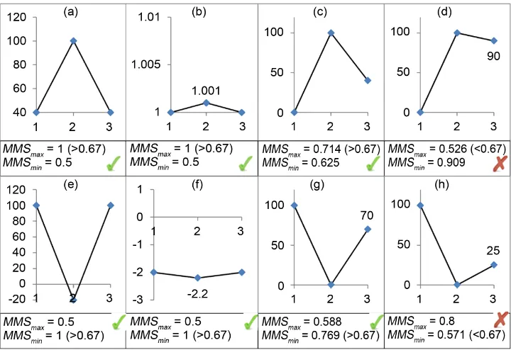
minimum of the three points is always considerably apart from the other two points. Plots (a), (b), and (c) of Figure 1 show situations that of MMSmax >2 3, where

maxi-mum is the peak. Plots (e), (f), and (g) in Figure 1 show situations that of

min 2 3

MMS > _{, where the minimum is the valley. However, Equation (4) does not}

al-ways successfully identify extrema, in other words if the identified point is the first or last point of a window, theoretically it cannot be considered as an extrema. Plots (d)

Figure 1. Plots (a), (b), (c), and (d) show different types of peaks and plots (e), (f), (g), and (h) show different types of valleys. For n = 3, value 2/n is 0.67. In all peaks except plot (d) MMSmax >

2/3 and in all valleys except plot (h) MMSmin < 2/3. “” corresponds to correct detections of

and (h) of Figure 1 show situations where neither a maximum nor a minimum repre-sents an extremum. Figure 1(d) shows a peak that of MMSmin >2 3 (identification of

a valley), this is a contradicting situation. Also, Figure 1(h) shows another failing situa-tion, where the plot shows a valley that of MMSmax >2 3 (identification of a peak).

This occurs because in both considered situations, the point has the highest deviation is the first point and not the middle point. Therefore, Equation (4) is not capable of iden-tifying extrema in such cases, thus handling these situations is required.

To address the aforementioned drawback, the MMS method was modified by con-sidering the middle point of the window. To have an exact middle point in a data win-dow the number of considered data points (n) must be odd. When n = 3 and amid is the

middle point of the window, substituting amax from Equation (1) by amid retrieves:

(

) (

)

max|mid mid min 3 min 3

MMS = a −a S a− ∗ _{. (5)}

Also, by replacing amin of Equation (2) by amid gives,

(

) (

)

min|mid max mid max 3 3

MMS = a −a a ∗ −S _{. (6)} Consider the situation,

max max|mid

MMS =MMS _{. (7)}

(

) (

) (

) (

)

max mid

a =a _{. (8)} Therefore, Equation (7) denotes the situation of a maximum at the middle point. Thus Equation (7) is a condition, independent of the value of MMS that can be used for identifying a peak.

Consider the situation:

min min|mid

MMS =MMS _{. (9)}

(

) (

) (

) (

)

min mid

a =a _{. (10)} Then Equation (9) denotes the situation of a minimum at the middle point. Thus, Equation (9) is a condition, independent of the value of MMS that can be used for iden-tifying a valley.

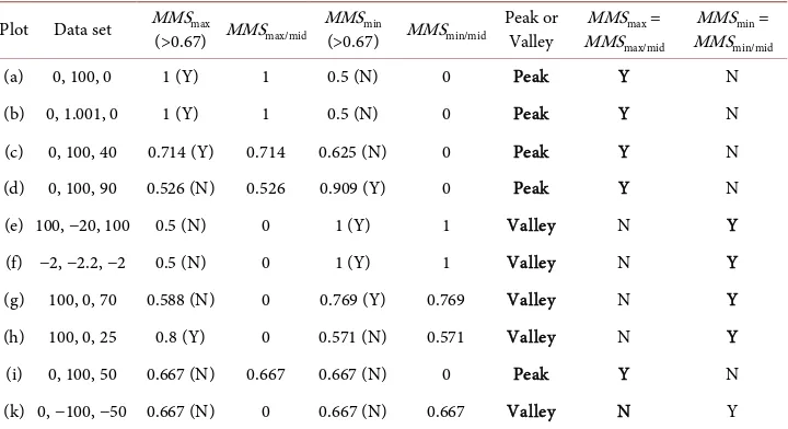
Therefore, when a window satisfies Equation (7) it implies that the middle point is a maximum and once a window satisfies Equation (9) it alternatively implies that the middle point is a minimum. Advancing the three point window by one data point makes it possible to locate all the extrema in a signal (Figure 2). Table 1 shows sample calculations of extrema detection procedure according to Equation (7) and Equation (9). The first eight value sets shown in Table 1 are the values in relation with the plots shown in Figure 1. Examples a, b, c, and d in Table 1 show calculation in relation with peak identification. In all these examples MMSmax =MMSmax|mid (Equation (7)) and

min min|mid

MMS ≠MMS (Equation (9)). Examples e, f, g, and h in Table 1 show calcula-tion in relacalcula-tion with valley identificacalcula-tion. In all these examples MMSmin =MMSmin|mid

Figure 2. Extrema detection process of proposed extrema identification method named as MMS max-min finder.

Table 1. Sample calculations of peak and valley detection process based new method (MMS max- min finder) for window size of three data points.

Plot Data set MMSmax

(>0.67) MMSmax/mid MMS_{(>0.67) MMS}min min/mid Peak or _{Valley MMS}MMSmax = max/mid

MMSmin = MMSmin/mid

(a) 0, 100, 0 1 (Y) 1 0.5 (N) 0 Peak Y N

(b) 0, 1.001, 0 1 (Y) 1 0.5 (N) 0 Peak Y N

(c) 0, 100, 40 0.714 (Y) 0.714 0.625 (N) 0 Peak Y N

(d) 0, 100, 90 0.526 (N) 0.526 0.909 (Y) 0 Peak Y N

(e) 100, −20, 100 0.5 (N) 0 1 (Y) 1 Valley N Y

(f) −2, −2.2, −2 0.5 (N) 0 1 (Y) 1 Valley N Y

(g) 100, 0, 70 0.588 (N) 0 0.769 (Y) 0.769 Valley N Y

(h) 100, 0, 25 0.8 (Y) 0 0.571 (N) 0.571 Valley N Y

(i) 0, 100, 50 0.667 (N) 0.667 0.667 (N) 0 Peak Y N

(k) 0, −100, −50 0.667 (N) 0 0.667 (N) 0.667 Valley N Y

k) show very special situations, where MMSmax, MMSmin, and 2/n are equal. In such

situations Equation (4) is undefined. However, even then extrema identification is pos-sible with Equation (7) and Equation (9). Since the proposed extrema detection method is based on the maximum, minimum, and sum of the series, the method was named as “MMS max-min finder”.

2.1. Identifying Dominating Extrema (Primary Filtering of Peaks and

Valleys)

(dominating valley) coincides with the middle point of an advancing window. Figure 3 shows an example of detecting dominating peaks in a window with odd number of data points (n = 7). When the number of data points per window increases, it allows for the possibility of more than one extremum in the considered window.

The plot in Figure 3 consists of seven data points and contains three peaks named A, B, and C. The peak A is the middle point of window Wn while peak B is the dominating

peak. Because of that point A is not recognise as a peak in window Wn. After advancing

Wn by two data points, Wn+2 appears. In the window Wn+2 the point B is the highest as

well as the middle point and the point B is recognized as a peak. Advancing Wn+2 by

two data points Wn+4 appears, where C becomes the middle point and due to the

influ-ence of point B it will not be recognized as a peak. This illustrates that the dominating extrema in a window remains undetected until the middle point of the window coin-cide with it whilst preventing identification of other small peaks and valleys.

The usage of windows with higher odd number of data points (e.g.: 5, 7, …) makes it possible to filter minor peaks and valleys. In contrast, if the methods in relation with height or width are used, the values are domain dependent and relative. Changing window size (W) is an absolute parameter and can be applied in any condition, espe-cially the situations that the domain conditions are unknown. However, this technique is not capable of filtering absolute small extrema, because the comparison is based on the existing extrema in the considered window. Furthermore, this technique is useful as a filter for removing relative small variations. Since the technique is based on the size of the window, the technique was named as “MMS-Window based filter” or (MMS-WBF).

Figure 3. Application of “MMS max-min finder” with window size of seven for locating maxi-mum point. In the window Wn the middle point is “A” and due to existence of point “B” in the

considered window, point “A” is not identified as the maximum point. Also, in the Wn+4 (the

window found after advancing by four data points) the point “C” is not identified as an extrema, due to existence of point “B” in the considered the window. In the Wn+2 the point “B” is the

2.2. Sharp and Gradual (Flat) Extrema Filtering

Extrema with starting and end points which are agreeing with y = c and having the middle point as the extremum can be considered as a symmetric extrema case. Plots (a) and (b) of Figure 4 show such symmetric extrema, which can be considered as the sim-plest symmetric form. Extrema shown in plots (c) and (d) of Figure 4 also fulfil the re-quirements of a perfect symmetric extrema. All the following equations in this section are based on the perfect extrema.

Consider a perfect maxima situation as shown in plot (c) of Figure 4. Here, all points are equal to amin (amin = c) except amax. Consider any perfect maximum situation with n

points, then n − 1 points are equal to amin, and amax ≠ c. The sum of the terms of such a

series can be expressed as:

(

)

min 1 max

n

S =a ∗ − +n a ₍₁₁₎

(

)

(

)

Consider a perfect minimum situation as shown in plot (d) of Figure 4. Here, all points of the series are equal to amax and amax = c except amin. Consider any perfect

maxima situation with n points. Then n − 1 points are equal to amax, and amin ≠ c. The

sum of the terms of such a series can be expressed as:

(

)

max 1 min

n

S =a ∗ − +n a ₍₁₃₎

(

)

(

)

If MMSmax MMSmin=RMm, then from (1) and (2),

(

) (

)

Mm n n

R = a ∗ −n S S −a ∗n .

When the maximum is detected as the peak, substituting in Equation (11) retrieves:

(

)

(

)

(

)

(

(

(

)

)

)

Mm

R = a ∗ −n a ∗ n− +a a ∗ n− +a −a ∗n

(

)

(

)

(

(

)

)

Mm

R = a ∗ −n a ∗ −n a +a a ∗ −n a +a −a ∗n

(

)

(

)

(

)

(

)

Mm

R = a −a ∗ −n a −a a −a

(

) (

)

(

)

(

)

Mm

R = a −a ∗ n− a −a

(

)

Mm

R = n−

(

)

max min 1

MMS MMS = n− ₍₁₅₎

In the same manner, if MMSmin/MMSmax = RmM, then from Equations (1), (2), and

(12), the minimum is detected as the valley,

(

)

mM

R = n−

(

)

min max 1

MMS MMS = n− ₍₁₆₎

The relations of Equation (15) and Equation (16) are crucial findings, which can be used to identify perfect extrema. When the extrema is not perfect, value of Equation (15) and Equation (16) is less than n − 1. Therefore, Equation (15) and Equation (16) can be used to identify perfect and non-perfect extrema. Also, perfect extrema are sud-den (sharp) extrema and non-perfect extrema can be considered as gradual extrema. Thereby, using Equation (15) and Equation (16) it is possible to filter sharp and gradual extrema.

After identifying a peak, by examining the ratio MMSmax/MMSmin it is possible to

de-termine degree of confidence of other points, the same applies for identifying a valley. Assume tMm_mM is the threshold value for determining sharp and gradual maxima, then

tMm_mM can be expressed as a k n∗ −

(

)

of n (e.g.: k=1

(

)

can be determined. The determination criteria (tMm_mM) of ratios MMSmax/MMSmin and

MMSmin/MMSmax are non-parametric and depend only on the number of data points in

the considered window. Since the method is also based on the maximum, the mini-mum, and the sum, the method was named as MMS-SG filter.

Figure 5 and Figure 6 show examples in relation with Equation (15) and Equation (16), respectively. In plots (a) and (b) of Figure 5, the ratio MMSmax/MMSmin = 6, which

is exactly equal to n − 1. This proves the correctness of Equation (15). In the same time, in plots (a) and (b) of Figure 6, the ratio MMSmin/MMSmax = 6 and proves the

correct-ness of Equation (16). All these plots exhibit either sudden peak or sudden valley. The corresponding ratios in relation with the plot (c) of Figure 5 andFigure 6are not equal to n − 1. However, the corresponding ratios are not very small. Therefore, these ex-trema can be considered as nearly sharp exex-trema. Nevertheless, corresponding ratios in relation with, plots (d) of Figure 5 and Figure 6 are very small and these extrema can be considered as gradual extrema.

2.3. High and Low Extrema Filtering

MMS-WBF and MMS-SG introduced in this work are capable identifying dominating, sharp and gradual extrema. However, these techniques are incapable of distinguishing the extrema with very small amplitude as shown in Figure 1(b) and Figure 1(f).

Figure 5. Plots (a), (b), (c), and (d) show four different types of peaks with window size seven (n = 7) where 2/n = 0.286. Ratios MMSmax/MMSmin and MMSmin/MMSmax are stated along with each

plot. Peaks in plots (a) and (b) are perfect peaks and the ratio MMSmax/MMSmin = 6 (i.e. n − 1).

Though, the dominating peak in plot (c) is not a perfect peak, ratio MMSmax/MMSmin is

con-sideribly high. The peak in plot (d) is a gradually developed peak and also not a perfect peak and the ratio MMSmax/MMSmin is very small. Therefore, consideration of ratio MMSmax/MMSmin is a

good criterion to distinguish sudden and gradual peaks.

Figure 6. Plots (a), (b), (c), and (d) show four different types of valleys with window size seven (n = 7) where 2/n = 0.286. Ratios MMSmax/MMSmin and MMSmin/MMSmax are stated along with each

plot. Valleys in plots (a) and (b) are perfect valleys and the ratio MMSmin/MMSmax = 6 (i.e. n − 1).

Though, the valley in plot (c) is not a perfect valley, ratio MMSmin/MMSmax is considerably high.

The valley in plot (d) is a gradually developed valley and also not a perfect valley and the ratio MMSmin/MMSmax is very small. Therefore, consideration of ratio MMSmin/MMSmax is a good

crite-rion for distinguishing between sudden and gradual (flat) valleys.

Then, Equation (13) can be expressed as:

(

)

min 1 min

n

S ≈a ∗ − +n a

(

)

min ; max

n

S ≈a ∗n <a ∗n

(

)

_ min min ;0 _ min 1

LH n LH

Figure 7. Two possible ways of existence of extremum for a data point; as a peak or as valley. Assume, except the extremum, all the other points are satisfying the y = c relation (perfect ex-trema). Then, extremum is the peak and all other points are equal to the minimum. In the same manner, when the extremum is a valley, valley is the minimum and all other points are equal to the maximum. If a peak is small it reaches to the minimum and when the valley is small it reaches to the maximum. This is the hypothesis for distinguishing small and high extrema.

If RLH_ min→1, it implies that the amin is very close to the other points (low crater),

consequently RLH_ min →0 implies that the amin is apart from the other points (high

crater).

In Equation (17), when the term amin is zero, the ratio RLH_min also becomes zero

de-spite of the influence of magnitude valley. Also, due to the influence of negative values Sn can be zero and RLH_min becomes invalid. Both these situations inhibit the

determina-tion of the real condidetermina-tion of the valley. To overcome the effect of negative values, the minimum value was deducted from all the terms of the data points in the window as expressed in Equation (18).

_ min.

i New i

a = −a a ₍₁₈₎ Even now it is possible to have a situation of amin = 0. To overcome this situation a

constant k, which is greater than zero, was added to each value. This transformation is applied in “Min-Max normalization” process [22][23]. When k = 1 thus Equation (18) becomes:

_ min 1

i New i

a = −a a + ₍₁₉₎

From Equation (17) and Equation (19),

(

)

(

)

(

)

_ min min min min

1

1 n 1

LH i

i

R a a n a a

=

= − + ∗

∑

_ min min

1 1 1

1

n n n

LH i

i i i

R n a a

= = =

 

= _ − + _



∑

∑

∑

(

)

_ min min ;0 LH_ min 1

LH n

(

)

(

)

_ min 1 ;0 _ min 1

LH n LH

R =n S + −a ∗n <R ≤ ₍₂₀₎

Then RLH_min expressed in Equation (20) can be considered as a robust method for

filtering valleys with low crater.

The peak shown in Figure 7 is a general situation of perfect peak. When a peak has a very small prominence, amax ≈ amin. Then Equation (11) can be expressed as:

(

)

max 1 max

n

S ≈a ∗ − +n a

(

)

max ; min

n

S ≈a ∗n >a ∗n

(

)

_ max max ; 0

LH n

R = a ∗n S > ₍₂₁₎

According to Equation (17), the ratio RLH_min has a well-defined upper limit (ceiling)

and lower limit (floor) because 0<RLH_ min ≤1. Nevertheless, in Equation (21), RLH_max

has no upper limit, and subjects only to a lower limit. Therefore, it is difficult to use RLH_max as a global criteria as RLH_min. The peak shown in Figure 7 can be considered as

the mirror image of a valley in Figure 7. Thus, it is possible to transform a peak to a valley, for that Equation (17) can be used for determining the peaks with high and low prominence using the same criteria Under the assumption that:

(

)

_ max min –

i New i

a = a +a a ₍₂₂₎ According to Equation (22),

(

)

(

)

value into the minimum, the minimum value into the maximum and intermediate val-ues into their complements. If the RLH_max is the corresponding ratio in relation with

high and low peaks identification, then, from Equation (21) and Equation (22), one can reach:

(

)

(

)

(

)

(

(

)

)

_ max max min max max min

1 n

LH i

i

R a a a n a a a

=

= + − ∗

_∑

(

)

(

(

)

)

_ max min 1 max min

n

LH i i

R = a ∗n

_∑

Even after the aforementioned transformation, it is still possible to have the influence of negative values. However, it can be resolved by using Equation (19). Then, from Equation (19),

(

)

(

)

(

(

) (

)

)

_ max min min max min min min min

1

1 n 1 1 1

LH i

i

R a a n a a a a a a

=

= − + ∗

∑

(

)

(

)

_ max max

1

1 n

LH i

i

R n a a

=

=

∑

(

)

(

)

_ max max 1 ;0 _ max 1

LH n LH

R =n a + ∗ −n S <R ≤ ₍₂₄₎

_ max 1 LH

R → _{implies that the amax is very close to other points (low prominence).}

Consequently RLH_ max →0 implies that the amax is apart from the other points (high

prominence).

Because the method is based on the maximum, minimum and the sum, the method was named as MMS-LH. Figure 8 elaborates the functionality of MMS-LH as a filtering method.

The filtration of sudden, gradual, low, and high extrema are derived based on a data set which satisfies the y = c relation (perfect extrema). However, in reality it is impossi-ble to always have perfect extrema. Therefore, by setting the threshold values in appro-priate situations, it is possible to filter the extrema in non-perfect conditions.

Extrema identification is performed after comparing two ratios in relation with maximum, minimum, middle point and sum. The threshold criteria for MMS-WBF and MMS-SG are values that are based on the number of data points (n). The threshold criterion for MMS-LH is a value between 0 and 1. Thus, all the determination criteria are totally non-parametric. However, combination of these methods leads to harvest more robust and reliable output. Figure 9 elaborates one possibility of combining all these methods for achieving reliable output.

All the algorithms were implemented using C++ in Net 2008 platform and tested with biogas data which were collected online form a biogas plant using NIR spectros-copy for a period of seven months with a frequency of twelve data points per day (i.e. every second hour). Among the different parameters, the H2 content measured in ppm

was selected, which has considerable amount of variations during the process. Data of each month was considered as a segment, where each segment consists of 350 - 400 data points. The proposed detection methods were applied on each segment with dif-ferent criteria. Furthermore, another data set of around 4800 data points, concentra-tions of volatile fatty acid (VFA), was selected for checking segmenting capabilities of the method.

Figure 9. One possible way of combining all the developed methods for har-vesting quality output.

3. Results and Discussion

3.1. Identifying Extrema

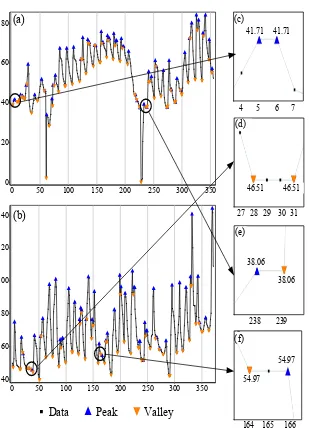
Figure 10. Two plots of H2 content of biogas data in two different months are presented

meas-ured in ppm. All the maxima in both the data sets ((a) and (b)) were identified by the new method with the window side is three (W = 3). Plots (c), (d), (e), and (f) show identification of special situations as extrema, even though they are existing derivative methods not consider as extrema situations.

Plot (e) and (f) of Figure 10 show other different situations, where it has consecutive minima and maxima of the same value. This also implies that the intermediate points have the same value ((f) of Figure 10). If consecutive maxima have same values and the order of occurrence is maximum then minimum, it can be considered as a discrete sad-dle region in an increasing data segment ((e) of Figure 10). In the same manner, if the two consecutive extrema have same value and the order of occurrence is minimum then maximum, it can be considered as a discrete saddle region in a decreasing data segment ((f) of Figure 10). Using the same criteria these detections can be excluded, if neces-sary.

Data Peak Valley

140

120

100

80

60

40

350 300 250 200 150 100 50 0

80

60

40

20

0

350 300 250 200 150 100 50 0

(b)

4 5 6 7

41.71 41.71

(c)

27 28 29 30 31 46.51 46.51

(d)

238 239 38.06

38.06

(e)

164 165 166

(f)

54.97

54.97

(a)

3.2. Identifying Dominating Extrema (Primary Filtering of Peaks and

Valleys)

The same two data sets shown in Figure 10 were filtered using MMS-WBF (MMS Window based filtering) method for identifying the dominant extrema using a window size of 9 (W = 9). Results of the detection process are shown in Figure 11 plots (a) and (b) demonstrate that the MMS-WBF was capable to identify 50% and 59% of all extrema as dominating extrema, respectively. However, out of the identified extrema in plots (a) and (b), there are 0.12% and 0.09% of small peaks which are identified as dominating extrema. These extrema cannot be visually justified as dominating extrema. Neverthe-less, numerically they are the dominating extrema in the considered window size. One possible option is to increase the window size, thus covering more data which enhances the capability of removing more non-dominating extrema. However, when W > 3, all

Figure 11. Plots (a) and (b) show the same data as plots (a) and (b) in Figure 10, filtered with MMS-WBF with a window size of nine data points (W = 9). MMS-WBF was capable of identify-ing 53% and 58% of all extrema as dominatidentify-ing extrema. However, MMS-WBF identified 0.12% and 0.09% of extrema in plots (a) and (b) as dominating extrema, which cannot be visually justi-fied as dominating extrema. Though those are cannot be justifies as dominating extrema, mathematically they are the dominating extrema in the considered window size. One possible option is to increase the window size, thus the window would cover more data points. This will remove more non-dominating extrema once a significant dominating extremum exists.

80

70

60

50

40

30

20

10

0

300 200

100 0

70

200 150

50

45 20

90

80

70

160 120

140

120

100

80

60

40

300 200

100 0

Data Peak Valley Correct _Filtering Incorrect _Filtering

(a)

the candidate points have not been checked. This is a disadvantage of increasing the window size for filtering non-dominating extrema. In plot (d) of Figure 11, at the end of the data set shows such an unidentified dominating peak due to W > 3 situation.

The combination of MMS max-min finder and MMS-WBF can be used in online data checking. For that, first the window size (W) has to be defined, and then the win-dow accumulates the data, after which the desired detection technique is applied and eventually the extrema are located. Subsequently, window is advanced by one data point and awaits the next data point. After the next point is captured, the extrema- check is performed again. This process is propagated throughout the process for locat-ing extrema in an online environment.

3.3. Sharp and Gradual (Flat) Extrema Filtering

Figure 12 shows the results in relation with sharp and gradual extrema detection per-formed based upon RMmand RmM as defined in Equation (15) and Equation (16),

re-spectively. Value of tMm_mM for RMm and RmM was set as 1 (k=1

(

)

of Figure 12 show the filtering of extrema, first with MMS-WBF for W = 3 and then with MMS-SG filter. Plot (c) and (d) of Figure 12 shows the filtering of extrema with MMS-WBF in the case of a window size of 9 (W = 9) and then with MMS-SG filter. When compared, plots (a) and (b) of Figure 12 show 78% and 77% less number of all extrema than number of extrema shown in plots (a) and (b) of Figure 10. When the W is small (W = 3) filter excludes some extrema seems to be very high (V1, P1, P2, and P3

shown in plots (a) and (b) of Figure 12), which can be considered as wrong detection. However, according to Equation (11) and Equation (13), rejections of those points are mathematically correct. This happens due to usage of small window size for extrema detection. Thus, one solution for overcoming this situation is to use lager window size.

Plots (c) and (d) in Figure 12 show identification of V1, P1, P2, and P3 after increasing

the window size to nine (W = 9). After applying large W (W = 9) almost all the flat ex-trema have been rejected. Even after increasing the W still exex-trema such as P4 are

re-maining, because W is not big enough to reject such points (i.e. in the selected window size, the extremum point is located significantly away from other points). In general, plots (c) and (d) of Figure 12 show 0.46% and 0.75% fewer extrema in comparison with plots (a) and (b) of Figure 12 and all the detections and rejections are agreed with the developed method. Therefore, the ratios MMSmax/MMSmin and MMSmin/MMSmax can be

considered as filtering criteria and a reliable technique for filtering sharp and gradual (flat) extrema.

3.4. High and Low Extrema Filtering

As per the results shown in Figure 10 and Figure 12 it is very clear that the “primary filtering” and consideration of MMSmax/MMSmin and MMSmin/MMSmax are not capable

Figure 12. Filtering of sudden and gradually developed (flat) extrema using MMS-SG technique. Data in plots (a) and (b) were first checked for extrema with a window of size three with MMS-WBF. Data in plots (c) and (d) were first checked for extrema with a window of size nine with MMS-WBF. Then ratios MMSmax/MMSmin and MMSmin/MMSmax considered and all

the plots were checked for sudden and gradually developed extrema with threshold value tMm_mM = 1. When the window size

is small, extrema such as V1, P1, P2, and P3 remain undetected. However, increasing the window size let those points to be

detected (plots (c) and (d)). Even after increasing the window size, points that have very small extrema such as P4 will de

de-tect as an extrema.

Before applying MMS-LH, data points (plots (a) and (b) of Figure 13) were first checked for extrema with a window size three with MMS-WBF and data in plots (c) and (d) of Figure 13 were first checked for extrema with a window size nine with MMS-WBF. Point V1 in Figure 13(a), which seems to be a valley with high crater, yet

remains as unidentified. To be qualified as an extrema with higher prominence or cra-ter, first, the extremum must be a perfect extremum. However, with W = 3, V1 is not a

perfect extremum. Therefore, the rejection is logical as well as mathematically correct. Nevertheless, in Figure 13(c), point V1 is identified as a valley, because the large

win-dow size (W = 9) makes V1 a nearly perfect extremum. Therefore, using W > 3 with

appropriate filter criteria the method can be used for filtering extrema with low and

80 60 40 20 0 350 300 250 200 150 100 50 0 80 60 40 20 0 350 300 250 200 150 100 50 0 140 120 100 80 60 40 350 300 250 200 150 100 50 0 140 120 100 80 60 40 350 300 250 200 150 100 50 0

Data Peak Valley

(a) (b)

(c) (d)

A

Figure 13. Filtering of low and high extrema using MMS-LH filtering technique. Data in plots (a) and (b) were first checked for extrema with a window of size three with MMS-WBF. Data in plots (c) and (d) were first checked for extrema with a window of size nine with MMS-WBF. Then RLH_max and RLH_min were considered and all the plots

were checked for low and high extrema with threshold value tLH = 0.05. When the window size is small, extrema

such as V1 remain undetected. The reason is for such detection is that the one point (point C) is located very close to

the extremum (extremum is not a perfect extremum). However, increasing the window size (W = 9) makes V1 a

nearly perfect extremum and detected in plot (c).

high prominence or crater.

3.5. Drawbacks of Using Large Window Size for Extrema Filtering

window is laid on a non-data region. Using a suitable padding, this part can be filled. For example, the entire data in non-data region in the start can be padded with starting value. Also, at the end suitable padding technique can be used to fill the part of the window in the non-data region.

3.6. Possibility of Use as a Data Segmentation Technique

Usually, dominating peaks and the valleys can be considered as turning points of a cer-tain property of a signal, if those dominating extrema are not outliers. Thus, dominat-ing peaks and valleys are good points for segmentdominat-ing a signal as well as identifydominat-ing gen-eral trends. Figure 14 shows an attempt to accomplish such a segmenting approach using the developed method. Figure 14 contains a data set with around 4600 data points and only the MMS-WBF (dominating extrema identification technique) tech-nique was applied as the filtering techtech-nique. For testing segmenting capabilities of the method, considerably large W was used (W = 155 in plot (a) and W = 255 in plot (b) of Figure 14). In both situations segmentation and general trend identification shows highly promising capabilities. Existences of more than one adjacent similar types of ex-trema violate the trend identification and segmentation (i.e. existence of maximum af-ter a maximum instead of minimum). Circled areas in plot (a) of Figure 14 show two such occurrences. However, removing unnecessary adjacent peaks or valleys while keeping singular important peaks or valleys, is one solution for overcoming this prob-lem. Thereby it is necessary to develop a methodology for removing less important ex-trema. Increasing the W is another way of overcoming the said drawback. Plot (b) of Figure 14shows situation of increased W and detection with less adjacent same type of

Figure 14. Usage of “MMSmax-min finder” as a segmentation technique and trend identification technique. Plot (a) and (b) use window size 155 and 255, respectively. When the window side is low (W = 155) segmentation and trend identification is distracted due to occurrence of adjacent same type extrema. In plot (a) such two occurrences were circled. Increasing the window size produces better segmentation as shown in plot (b). However, this leads to ignore some trends as circled in plot (b).

7

6

5

4

3

2

1_{0 500 1000 1500 2000 2500 3000 3500 4000 4500}

7

6

5

4

3

2

1

4500 4000 3500 3000 2500 2000 1500 1000 500 0

Data

Segment points

extrema than plot (a) of Figure 14. However, this technique lead to ignorance of some features in the signal as circled in plot (b) of Figure 14. Therefore, determining of proper W is an essential factor for better identification of segments as well as trends. Nevertheless, the method can be used for at least fast segmentation and trend identifi-cation method.

4. Conclusion

The introduced extrema finding method named as “MMS Max-Min finder” and three different extrema filtering methods named as MMS-Window Based Filter (MMS- WBF), MMS sharp and gradual extrema filter (MMS-SG), and MMS low high extrema filter (MMS-LH) are non-parametric. Therefore, filtering can be done without consid-ering domain dependent parameters such as height and width of an extremum. Results prove that the detection is capable of identifying all the extrema with 0% error. When the window size is nine (W = 9) MMS-WBF reported 0.12% and 0.09% wrong detec-tions. However, a combination of MMS-WBF and MMS-LH filter with window size nine (W = 9) was capable of eliminating the error. Despite of the dynamic nature of the data, the results were consistent and robust for the same detection criteria. Thus, using proper window size, it is possible to achieve robust and consistent outcome with dy-namic data such as biogas data. Furthermore, MMS-WBF shows promising outcome in the direction of segmenting and trend identification of signals. Hence, MMS-WBF can be enhanced as a segmenting and trend identification technique.

Acknowledgements

This work was supported by the German Research Foundation (DFG) and the Technic-al University of Munich (TUM) in the framework of the Open Access Publishing Pro-gram. Also, we are grateful to the German Academic Exchange Service (Deutscher Akademischer Austauschdienst, DAAD) for providing a scholarship to KKLB Adikaram during the research period.

References

[1] Mavron, V.C. and Phillips, T.N. (2007) Maxima and Minima. In: Mavron, V.C. and Phil-lips, T.N., Eds., Elements of Mathematics for Economics and Finance, Springer, London, 137-158.

[2] Sande, H.V., Henrotte, F. and Hameyer, K. (2004) The Newton-Raphson Method for Solv-ing Non-Linear and Anisotropic Time-Harmonic Problems. The International Journal for Computation and Mathematics in Electrical and Electronic Engineering, 23, 950-958.

http://dx.doi.org/10.1108/03321640410553373

[3] Chioua, M., Srinivasan, B., Guay, M. and Perrier, M. (2007) Dependence of the Error in the Optimal Solution of Perturbation-Based Extremum Seeking Methods on the Excitation Frequency. The Canadian Journal of Chemical Engineering, 85, 447-453.

http://dx.doi.org/10.1002/cjce.5450850407

http://dx.doi.org/10.1016/S0377-0427(99)00088-6

[5] Gilgen, H. (2006) Univariate Time Series in Geosciences: Theory and Examples. Springer, Berlin.

[6] Zou, H.-F., Zhang, Y.-K. and Lu, P.-C. (1991) The Prediction of the Peak Width at Half Height in HPLC. Chinese Journal of Chemistry, 9, 237-244.

http://dx.doi.org/10.1002/cjoc.19910090307

[7] Antoniadis, A., Bigot, J. and Lambert-Lacroix, S. (2010) Peaks Detection and Alignment for Mass Spectrometry Data. Journal de la Société Française de Statistique, 151, 17-37.

[8] Jeffries, N. (2005) Algorithms for Alignment of Mass Spectrometry Proteomic Data. Bioin-formatics, 21, 3066-3073. http://dx.doi.org/10.1093/bioinformatics/bti482

[9] Sauve, A.C. and Speed, T.P. (2004) Normalization, Baseline Correction and Alignment of High-Throughput Mass Spectrometry Data. Proceedings Gensips.

[10] Mtetwa, N. and Smith, L.S. (2006) Smoothing and Thresholding in Neuronal Spike Detec-tion. Neurocomputing, 69, 1366-1370. http://dx.doi.org/10.1016/j.neucom.2005.12.108

[11] Tzallas, A.T., Oikonomou, V.P. and Fotiadis, D. (2006) Epileptic Spike Detection Using a Kalman Filter Based Approach. IEEE Engineering in Medicine and Biology Society Confe-rence, 1, 501-504. http://dx.doi.org/10.1109/iembs.2006.260780

[12] Gelb, A. (1974) Applied Optimal Estimation. MIT Press, Boston.

[13] Shim, B., Min, H. and Yoon, S. (2009) Nonlinear Preprocessing Method for Detecting Peaks from Gas Chromatograms. BMC Bioinformatics, 10, 378.

http://dx.doi.org/10.1186/1471-2105-10-378

[14] Scholkmann, F., Boss, J. and Wolf, M. (2012) An Efficient Algorithm for Automatic Peak Detection in Noisy Periodic and Quasi-Periodic Signals. Algorithms, 5, 588-603.

http://dx.doi.org/10.3390/a5040588

[15] Györfi, L., Kohler, M., Krzyzak, A. and Walk, H. (2006) A Distribution-Free Theory of Nonparametric Regression. Springer, New York.

[16] Roberts, S.J. (1997) Parametric and Non-Parametric Unsupervised Cluster Analysis. Pattern Recognition, 30, 261-272. http://dx.doi.org/10.1016/S0031-3203(96)00079-9

[17] Wasserman, L. (2006) All of Nonparametric Statistics. Springer, New York.

[18] Kothari, C.R. (2004) Research Methodology: Methods and Techniques. New Age Interna-tional (P) Limited,Delhi.

[19] Li, J., Ray, S. and Lindsay, B.G. (2007) A Nonparametric Statistical Approach to Clustering via Mode Identification. Journal of Machine Learning Research, 8, 1687-1723.

[20] Adikaram, K.K.L.B., Hussein, M.A., Effenberger, M. and Becker, T. (2014) Outlier Detec-tion Method in Linear Regression Based on Sum of Arithmetic Progression. The Scientific World Journal,2014, Article ID: 821623. http://dx.doi.org/10.1155/2014/821623

[21] Adikaram, K.K.L.B., Hussein, M.A., Effenberger, M. and Becker, T. (2015) Universal Linear Fit Identification: A Method Independent of Data, Outliers and Noise Distribution Model and Free of Missing or Removed Data Imputation. PLoS ONE, 10, e0141486.

http://dx.doi.org/10.1371/journal.pone.0141486

[22] Han, J., Kamber, M. and Pei, J. (2006) Data Mining, Southeast Asia Edition: Concepts and Techniques. Elsevier Science, Amsterdam.