Three-Dimensional Simulations with Fields and Particles
in Software and Inflector Designs
Branislav Radjenović1, Marija Radmilović-Radjenović1, Petar Beličev2
1Institute of Physics, University of Belgrade, Belgrade, Serbia; 2Vinča Institute of Nuclear Science, University of Belgrade, Belgrade, Serbia.
Email: [email protected]
Received June 1st, 2013; revised July 3rd, 2013; accepted July 12th, 2013
Copyright © 2013 Branislav Radjenovićet al. This is an open access article distributed under the Creative Commons Attribution License, which permits unrestricted use, distribution, and reproduction in any medium, provided the original work is properly cited.
ABSTRACT
Particles and fields represent two major modeling paradigms in pure and applied science at all. In this paper, a method- ology and some of the results for three-dimensional (3D) simulations that include both field and particle abstractions are presented. Electromagnetic field calculations used here are based on the discrete differential form representation of the finite elements method, while the Monte Carlo method makes foundation of the particle part of the simulations. The first example is the simulation of the feature profile evolution during SiO2 etching enhanced by Ar + /CF4 non-equilib- rium plasma based on the sparse field method for solving level set equations. Second example is devoted to the design of a spiral inflector which is one of the key devices of the axial injection system of the VINCY Cyclotron.
Keywords: Fields; Particles; Simulations; Finite Elements; Inflector; Profile Evolution; Level Set Method
1. Introduction
As already pointed out, fields and particles are two the
most important modeling paradigms in pure and applied science at all. Particles are primarily used in one of the two ways in large scientific applications. The first one is to track sample particles to gather statistics that describe the conditions of a complex physical system. Particles of this kind are often referred to as “tracers”. The second one is to perform direct numerical simulation of systems that contain discrete point-like entities such as ions or molecules. In both scenarios, the application contains one or more sets of particles. Each set has some data as- sociated with it that describes its members’ characteris- tics, such as charge, mass or momentum. The state of the physical system is defined by these data [1].
Particles typically exist in a spatial domain, and they may interact directly with one another or with field quantities defined on that domain. A field, on the other hand, defines a set of values on a region of space. In order to specify a field one must specify the locations at which the field’s values are defined, and describe what happens at the boundaries of that region in space. For this purpose we use meshes which are discrete represen- tations of the physical domains. Particle abstractions are usually designed to be used in conjunction with fields.
Some types of interpolators are used as the glue that bind these together, by specifying how to calculate field val- ues at particle (or other) locations that not happen to lie exactly on mesh points. Interpolators are used to gather values to specific positions in a field’s spatial domain from nearby field elements, or to scatter values from such positions into the field.
In this paper we present two examples of the simula- tions of this type, different in their origin but sharing the same software design concept and implementation com- ponents. The first is from the area of the applications of the plasma technologies in microelectronic circuits ma- nufacturing. The second is a part of the ongoing work on the design of the spiral inflector for the VINCY Cyclo- tron.
2. Software Design Issues
community have largely been unsuccessful until recently. However, recent advances in software technology signify that the hard to get goal of increased high-performance scientific programming productivity is possible.
Although Object-Oriented Programming itself was not the main reason for the improved productivity the busi- ness community (the rise in productivity comes from the use of Object-Oriented Design and Component-Based Programming), the choice of the programming language is of the utmost importance. Development of complex scientific applications requires GUI toolkits, numeric li- braries, graphical facilities, libraries for interfacing with code written in other languages, etc. Many scientific pro- grammers and researchers still dream of a general-pur- pose language that is so expressive, elegant, and efficient that it can cover all needs without significant inconven- iences. However, no current language can satisfy all these requirements natively, and there is no a research language that could possibly do that in the short-to-me- dium term.
Our simulation framework (written in C++) is based on
Fltk library [2] for building GUI elements, Vtk toolkit [3] for 3D visualization needs, and Pthreads library [4] for managing multiple execution threads. Additional librar- ies and toolkits are used depending on the specific re- quirements of the particular applications.
3. Electromagnetic Field Calculations
In this approach the scalar electrostatic potential is a 0- form, the electric and magnetic fields are 1-forms, the electric and magnetic fluxes are 2-forms, and the scalar charge density is a 3-form. The basic operators are the exterior (or wedge) product, the exterior derivative, and the Hodge star. Precise rules (i.e. a calculus) prescribe how these forms and operators can be combined. In this modern geometrical approach to electromagnetics the fundamental conservation laws are not obscured by the details of coordinate system dependent notation. By working within the discrete differential forms framework, we are gauranteed that resulting spatial discretization schemes are fully mimetic [5,6].
The calculations of the electric fields in this paper are performed by integrating a general finite element solver GetDP [7,8] in our simulation framework. GetDP is a thorough implementation of discrete differential forms calculus, and uses mixed finite elements to discretize de Rham-type complexes in one, two and three dimensions. Meshing of the computational domain is carried out by TetGen tetrahedral mesh generator [9]. TetGen generates the boundary constrained high quality (Delaunay) meshes, suitable for numerical simulation using finite element and finite volume methods. As a part of the post-process- ing procedure the electric fields, obtained on the unstruc-
tured meshes, are recalculated on the Cartesian rectangu- lar domains containing the regions of the particles move- ment. In this manner, the electric field on the particles could be calculated by simple trilinear interpolation.
4. Simulation of Etching Profile Evolution
Refined control of etched profile in microelectronic de- vices during plasma etching process is one of the most important tasks of front-end and back-end microelectro- nic devices manufacturing technologies. The profile sur- face evolution in plasma etching, deposition and lithogra- phy development is a significant challenge for numerical methods for interface tracking itself. Level set methods for evolving interfaces [10,11] are specially designed for profiles which can develop sharp corners, change topol- ogy and undergo orders of magnitude changes in speed. They are based on a Hamilton-Jacobi type equation [12] for a level set function using techniques developed for solving hyperbolic partial differential equations. A sim-ple model of Ar + /F etching process that includes only
pure chemical and ion-enhanced chemical etching me- chanisms is presented in details.
Sparse Field Level Set Method
The basic idea behind the level set method is to represent the surface in question at a certain time t as the zero level set (with respect to the space variables) of a certain func-
tion φ(t, x), the so called level set function. The initial
surface is given by {x|φ(0, x) = 0}. The evolution of the
surface in time is caused by “forces” or fluxes of par- ticles reaching the surface in the case of the etching pro- cess. The velocity of the point on the surface normal to the surface will be denoted by V(t, x), and is called ve- locity function. For the points on the surface this function is determined by physical models of the ongoing pro- cesses; in the case of etching by the fluxes of incident particles and subsequent surface reactions. The velocity function generally depends on the time and space va- riables and we assume that it is defined on the whole simulation domain. At a later time t > 0, the surface is as
well the zero level set of the function φ(t, x), namely it
can be defined as a set of points {x∈ℜn|φ(t, x) = 0}.
This leads to the level set equation
H t, x
t
0,
(1)
in the unknown function φ(t, x), where φ(0, x) = 0 de-
face must be extracted from this grid. In order to apply
the level set method a suitable initial function φ(0, x) has
to be defined first. The natural choice for the initializa- tion is the signed distance function of a point from the given surface. This function is the common distance
function multiplied by −1 or +1 depending on which side
of the surface the point lies on. As already stated, the val- ues of the velocity function are determined by the physi- cal models. In the actual numerical implementation Equa- tion (1) is represented by the upwind finite difference schemes (see ref. [10] for the details) that requires the values of this function at the all grid points considered. In reality the physical models determine the velocity func- tion only at the zero level set, so it must be extrapolated suitably at grid points not adjacent to the zero level set. Several approaches for solving level set equations exist which increase accuracy while decreasing computational effort. They are all based on using some sort of adaptive schemes. The most important are narrow band level set method [10,11], widely used in etching process modeling tools, and recently developed sparse-filed method [13], implemented in medical image processing ITK library [14]. The sparse-field method use an approximation to the distance function that makes it feasible to recompute the neighborhood of the zero level set at each time step. In that way, it takes the narrow band strategy to the ex- treme. It computes updates on a band of grid points that is only one point wide. The width of the neighborhood is such that derivatives for the next time step can be calcu- lated.
Here we will present some calculations illustrating our approach for etching profile evolution simulation. All the
calculations are performed on 128 × 128 × 384 rectan-
gular grid [15]. The initial profile surface is a rectangle
deep with dimensions 0.1 × 0.1 × 0.1 μm. Above the
profile surface is the trench region. From its top the par- ticles involved in etching process come from, while bel- low is the non-etched material. The actual shape of the initial surface can be described using simple geometrical abstractions. In the beginning of the calculations this de- scription is transformed to the initial level set function using fast marching method [10]. The evolution of the et- ching profile surface with time is shown in the follow- ing figures. In Figure 1(a) the results obtained for a test calculation performed with constant velocity function V = V0 = 5 nm/s (purely isotropic etching case) are shown. It is supposed that only the bottom surface could be etched; i.e. that the top and the vertical surfaces belong to photo-resist layer. Behavior of the etching profile is as expected.
In the case of the ion enhanced chemical etching the dependence of the surface velocity on the incident angle
is simple [16]: V = V0 cosθ. The pure chemical etching
velocity, or more precisely the etching yield, does not
(a)
(b)
Figure 1. (a) Isotropic and (b) anisotropic etching-feature profiles at t = 0, t = 5 s, t = 10 s, t = 15 s.
depend on the incident angles. This case can be safely treated by the upwind scheme and using the Lax-Frie- drichs scheme would lead to unnecessary rounding of the profile surface. The high aspect ratio (depth/width) etch- ing is a common situation in semiconductor technologies. The evolution of the etching profile, when etching rate is
proportional to cos(θ), is presented in Figure 1(b). This
is the simplest form of angular dependence, but it de- scribes the ion enhanced chemical etching process cor- rectly [16]. In this case we expect that the horizontal sur- faces move downward, while the vertical ones stay still. This figure shows that it with optimal amount of smoo- thing gives minimal rounding of sharp corners, while preserving the numerical stability of the calculations. Ac- tually, this is one of the most delicate problems in the etching profile simulations.
[image:3.595.327.517.82.310.2]0 20 40 60 80 100 120 140 160 0,1
1 10
80 60 40 20 0
1 10 100
Angle [o]
An
gl
e di
strib
u
tio
n
fun
c
tion
[1
0
9
]
E
n
er
g
y
d
istr
ibu
ti
on
fu
ncti
on
[
1
0
9 ]
Energy [eV]
EEDF IEDF
[image:4.595.352.496.83.360.2]EADF IADF
Figure 2. Electrons (EEDF, EADF) and ions (IEDF, IADF) energy and angular distribution functions.
fluxes incident on the profile surface. Our simulation concept [20] is similar in spirit to the 2D simulations pre- sented in [21,22] and especially [23], where charging ef- fects in 3D rectangular trench were analyzed. Monte Carlo technique is the only feasible method for calculat- ing particle fluxes in 3D geometries. Trench wall charg- ing strongly influences the charged particles motion and, consequently, particle fluxes which themselves deter- mine the local etching rates.
Since the trench boundaries have no regular (rectan- gular) shape in our simulation, finite element calculations was used for the calculation of the electric field. As the etching profile is not known in advance (it is a result of the calculations itself), the problem of meshing is ex- tremely difficult. In Figure 3 the electrostatic potential map is shown for a test case calculation, for illustrating purposes only. Electric field obtained in that way is used in standard leap-frog particle moving scheme.
5. Inflector Design
[image:4.595.64.284.86.265.2]This part work is related to the activities concerning the design of the spiral inflectors for this facility, which is the second example of coupled field and particle simula- tions treated in this paper [24]. The main roles of the in- flector are to bend the injeced ion beam from its initial direction onto the cyclotron’s madian plane and, together with the optical elements in the transport line, to match the beam emittance to the cyclotron’s acceptance. The electrostatic inflector consists of two biased and two grounded electrodes. The electric field produced by these electrodes exerts a force on the ions, simultaneously bending and focusing the beam. The design of an electro- static inflector is complicated by the fact that in addition to the electrostatic force produced by its electrodes, the ions are also subjected to a magnetic force produced by
Figure 3. An example of the electrostatic potential map of the charged feature profile.
the simultaneously bending and focusing the beam. The design of an electrostatic inflector is complicated by the fact that in addition to the electrostatic force produced by its electrodes, the ions are also subjected to a magnetic force produced by the magnetic field near the center of the cyclotron. This effect must be taken into account in designing the inflector. Different types of inflectors have been devised [24-27] for inflecting the axially injected ion beam into the cyclotron median plane. In modern, variable energy, multi-particle, compact cyclotrons, the minimal gap between the magnetic poles tends to be very small (few centimeters-to provide high flutter and high magnetic circuit efficiency). This fact imposes severe re- strictions on inflector dimensions, as well as specific de- mands concerning its optical properties. Owing to its fle- xibility and relatively low voltage needed for its opera- tion, the electrostatic spiral inflector has become widely used in the multi-particle compact cyclotrons. Due to the complexity of the shape of its electrodes, this particular type of inflector has been chosen as illustrative (see Fig- ure 4).
The ion trajectories are calculated by solving Newton- Lorenz equations of motion using Boris integrator scheme [1], since magnetic field must be taken into account also.
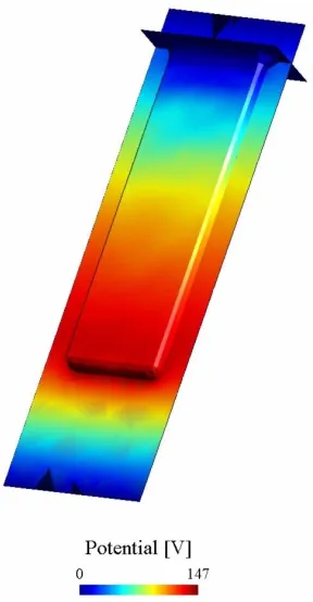
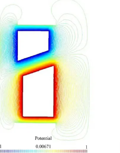
In Figure 5 an electrostatic potential map at the exit
plane of the inflector is shown. The voltages applied to
the upper and the lower electrodes are taken to be −1 V
Figure 4. Mechanical drawing of the spiral inflector.
Figure 5. Electrostatic potential map at the exit plane of the spiral inflector.
6. Conclusion
In this paper we presented some results of two different types of combined particle-field simulations (based on the unified software framework), in which the authors are involved. The first is connected with the applications of the plasma etching technologies in microelectronic cir- cuits manufacturing. Obtained results show that more realistic calculations should include the effects of poly- mer deposition, profile charging, more complex surface reactions set, as well as better statistic (greater number of
particles) in the Monte Carlo step of the calculations, which is now limited by the available computational re- sources. Another is a part of the ongoing work on the design of the spiral inflector for the VINCY Cyclotron. In present phase this simulations are preliminary, and more comprehensive analysis that includes the detailed maps of central region magnetic field, particle bunches and interparticle interaction is necessary.
7. Acknowledgements
The present work has been supported by O171037, III 41011 and III45006 Projects of Ministry of Education and Science, Serbia.
REFERENCES
[1] G. C. Birdsall and A. Langdon, “Plasma Physics via Computer Simulation,” McGraw-Hill, New York, 1985. [2] Fltk. http://www.fltk.org
[3] Vtk. http://www.vtk.org
[4] Pthreads. http://sourceware.org/pthreads-win32
[5] A. Bossavit, “Computational Electromagnetism,” Acade- mic Press, Boston, 1998.
[6] K. Warnick, R. Selfridge and T. Arnold, “Teaching Elec- tromagnetic Field Theory Using Differential Form,” IEEE Transactions on Education, Vol. 40, No. 1, 1997, pp. 53- 68. doi:10.1109/13.554670
[7] C. Geuzaine, “High Order Hybrid Finite Element Schemes for Maxwell’s Equations Taking Thin Structures and Global Quantities into Account,” Ph.D. Thesis, Universite de Liege, Liege, 2001.
[8] GetDP. http://www.geuz.org/getdp [9] TetGen. http://tetgen.berlios.de
[10] J. Sethian, “Level Set Methods and Fast arching Methods: Evolving Interfaces in Computational Geometry, Fluid Mechanics, Computer Vision and Materials Sciences,” Cambridge University Press, Cambridge, 1998.
[11] S. Osher and R. Fedkiw,“Level Set Method and Dynamic Implicit Surfaces,” Springer, New York, 2002.
[12] L. Evans, “Partial Differential Equations,” American Ma- thematical Society, Providence, 1998.
[13] R. Whitaker, “A Level-Set Approach to 3D Reconstruc- tion From Range Data,” International Journal of Com- puter Vision, Vol. 29, No. 3, 1998, pp. 203-231.
doi:10.1023/A:1008036829907
[14] Insight Segmentation and Registration Toolkit. http://www.itk.org
[15] B. Radjenović, J. K. Lee and M. Radmilović-Radjenović, “Sparse Field Level Set Method for Non-Convex Hamil- tonians in 3D Plasma Etching Profile Simulations,” Com- puter Physics Communications,Vol. 174, No. 2, 2006, pp. 127-132. doi:10.1016/j.cpc.2005.09.010
[image:5.595.65.268.312.570.2]Sons, Inc., Hoboken, 1994.
[17] C. K. Birdsall, “Particle-in-Cell Charged-Particle Simula- tions, Plus Monte Carlo Collisions with Neutral Atoms,” IEEE Transactions on Plasma Science, Vol. 19, No. 2, 1991, pp. 65-85. doi:10.1109/27.106800
[18] J. P. Verboncoeur, M. V. Alves, V. Vahedi and C. Bird- sall, “Simultaneous Potential and Circuit Solution for 1D Bounded Plasma Particle Simulation Codes,” Journal of Computational Physics, Vol. 104, No. 2, 1993, pp. 321- 328. doi:10.1006/jcph.1993.1034
[19] H. C. Kim, F. Iza, S. S. Yang, M. Radmilović-Radjenović and J. K. Lee, “Particle and Fluid Simulations of Low- Temperature Plasma Discharge: Benchmarks and Kinetic Effects,” Journal of Physics D: Applied Physics,Vol.38, No. 19, 2005, pp. R283-R301.
doi:10.1088/0022-3727/38/19/R01
[20] B. Radjenović and J. K. Lee, “3D Feature Profile Evolu- tion Simulation for SiO2 Etching in Fluorocarbon Plasma,” Proceeding of the XXVIIth ICPIG, Eindhoven, 18-22 July 2005.
[21] G. Hwang and K. Giapis, “On the Origin of the Notching Effect during Etching in Uniform High Density Plasmas,” Journal of Vacuum Science and Technology, Vol. B15, No. 1, 1997, pp. 70-87.
[22] A. Mahorowala and H. Sawin, “Etching of Polysilicon in Inductively Coupled Cl2 and HBr Discharges. IV. Calcu- lation of Feature Charging in Profile Evolution,” Journal of Vacuum Science and Technology, Vol. B20, No. 3, 2002, pp. 1084-1095.
[23] H. S. Park, S. J. Kim, Y. Q. Wu and J. K. Lee, “Effects of Plasma Chamber Pressure on the etching of Micro Struc- tures in SiO2 with the Charging Effects,” IEEE Transac- tions on Plasma Science, Vol. 31, 2003, pp. 703-710. doi:10.1109/TPS.2003.815245
[24] N. Nešković, et al., “Status Report on the VINCY Cyclo- tron,” Nukleonika, Vol. 48, 2003, pp. S135-S139. [25] W. B. Powell and B. L. Reece,“Injection of Ions into a
Cyclotron from an External Source,” Nuclear Instruments and Methods,Vol. 32, No. 2, 1965, pp. 325-332. doi:10.1016/0029-554X(65)90531-8
[26] J. L. Belmont and J. L. Pabot, “Study of Axial Injection for the Grenoble Cyclotron,” IEEE Transactions on Nu- clear Sciences, Vol. NS-13, 1966, pp. 191-193.
doi:10.1109/TNS.1966.4324204