Cooperating firms in inventive and absorptive research

Munich Personal RePEc Archive

Cooperating firms in inventive and

absorptive research

Ben Youssef, Slim and Breton, Michèle and Zaccour, Georges

Manouba University, ESC de Tunis and LAREQUAD, Tunisia,

GERAD, HEC Montréal, Canada, GERAD, HEC Montréal, Canada

Cooperating Firms in Inventive and Absorptive

Research

Slim Ben Youssef

_·

Mich`

ele Breton

_·

Georges Zaccour

December 5, 2011

Abstract

We consider a duopoly competing in quantity, where firms can invest in both innovative and absorptive R&D to reduce their unit production cost, and where they benefit from free R&D spillovers between them. We analyze the case where firms act non cooperatively and the case where they cooperate by forming a research joint venture. We show that, in both modes of play, there exists a unique symmetric solution. We find that the investment in innovative R&D is always higher than in absorptive R&D. We also find that the value of the learning parameter has almost no impact on innovative R&D, firms profits, consumer’s surplus and social welfare. Finally, differences in investment in absorptive research and social welfare under the two regimes are in opposite directions according to the importance of the free spillover.

Key Words: Innovative R&D· Absorptive R&D·Learning Parame-ter_·Spillover_·Research Joint Venture.

Slim Ben Youssef

Manouba University, ESC de Tunis and LAREQUAD, Tunisia

Mich`ele Breton

GERAD, HEC Montr´eal, Canada

Georges Zaccour (corr. author)

Chair in Game Theory and Management, GERAD, HEC Montr´eal, Canada

1

Introduction

In this paper, we consider a duopoly where firms can invest both in innovative (or original) and absorptive research and development (R&D) to reduce their unit production cost. We suppose the existence of free and exogenous R&D spillovers, that is, a firm cannot fully appropriate the knowledge developed in its laboratory. However, for a firm to benefit from rival’s innovative R&D, it must invest in absorptive capacity, e.g., hire technical staff to adapt the rival’s knowledge to its context. The duopoly game is played in two stages: In the first stage, firms choose their investment levels in R&D, and in the second stage they compete in quantity on the market. We consider two cases. In the first case, the firms act non-cooperatively, while in the second case, they cooperate in both types of research by forming a research joint venture (RJV). Interestingly, we show that under both modes of play, the sub-game perfect equilibrium is unique. We then characterize and compare the cooperative and non-cooperative R&D equilibrium strategies and outcomes.

competi-exist. For the latter, they found that total profits are sometimes higher with R&D competition than with RJV.

The above-mentioned references all assume that R&D spillovers are exoge-nous and cost less. A second stream of literature considers that, to benefit from the rival’s R&D, a firm must acquire absorptive capacity. Cohen and Levinthal [7] were the first to introduce the concept of absorptive capacity in the R&D literature. They showed that investment in R&D develops the firm’s ability to identify, assimilate, and exploit knowledge from the environment, which they termed “learning” or “absorptive” capacity. Poyago-Theotoky [8] showed that, when information spillovers are endogenized, non cooperating firms never dis-close any of their knowledge, whereas they always share their full knowledge when they cooperate in R&D. Kamien and Zang [9] found that, when firms cooperate in R&D, they choose identical R&D approaches, while they choose firm-specific R&D approaches otherwise, unless there is no danger of exogenous spillovers. In contrast, Wiethaus [10] showed that competing firms do choose identical R&D approaches in order to maximize the flow of knowledge between them.

ratio of innovative cost reduction to output. Hammerschmidt [17] considered a two-stage game in which R&D plays a dual role: first, it generates new knowl-edge; and second, it develops a firm’s absorptive capacity. She found that firms invest more in R&D to strengthen their absorptive capacity when the spillover parameter is higher. Finally, Kannianinen and Stenbacka [18] showed that there is an under investment in imitation from a social point of view when imitation leads to sufficiently intense competition.

Our paper is principally related to this third stream of literature. We con-sider the investment in absorptive capacity as a decision separate from the investment in innovative R&D. The two decisions are however related, as invest-ment in absorptive capacity allows the firms to increase the spillover from the rival’s research. Our main contributions are the introduction of a free spillover parameter along with a learning (or absorptive) parameter, the comparison of non-cooperative and cooperative outcomes, and the analysis of the impact on firms profits and on social welfare of parameter values and modes of play.

More specifically, we address the following questions:

1. How do investment levels in innovative and absorptive research compare under cooperation and non-cooperation in R&D?

2. What is the impact of the free spillover and learning parameters on strate-gies and outcomes?

3. Does cooperation in R&D improve profits, consumers’ surplus or welfare?

We obtain some new and non obvious results. Indeed, contrary to the results obtained when decisions in absorptive and innovative research are not dissoci-ated, as in [11], we find that an increase in the efficiency of absorptive research investments has almost no impact on innovative R&D investments, firms’ profits, consumers’ surplus and social welfare. We also find that when the free spillover is low, investment in absorptive R&D, consumers’ surplus and social welfare are higher under non-cooperation than under a RJV. This challenges a result in [4] stating that a RJV can raise welfare even in the absence of spillovers.

A third interesting result, in line with a finding of [17] in a non-cooperative setting, is that investment in innovative R&D is always higher than in absorptive R&D, in both the cooperative and non-cooperative cases, even when investment costs for innovation are much higher than for absorption capacity.

prof-investments in a RJV. This last result carries a priori a non-obvious message. Indeed, under cooperation, one could presume that when the free spillover de-creases, firms are tempted to compensate by increasing their investment in ab-sorption capacity, but our computations show that this is not the case.

The rest of the paper is organized as follows. Section 2 presents the basic model and Section 3 the market equilibrium. Section 4 characterizes the unique symmetric equilibrium in the non-cooperative case and Section 5 characterizes the unique equilibrium solution when the firms cooperate in R&D. Section 6 presents and discusses numerical illustrations and Section 7 briefly concludes.

2

The model

We consider a duopolistic industry producing a homogeneous good sold on a market having the following linear inverse demand function:

p(qi, qj) =λ−b(qi+qj), λ >0, b >0, i, j∈ {1,2}, j6=i.

Firms are symmetrical and can invest in R&D to decrease their per-unit production cost. We distinguish between two types of R&D efforts, namely, innovative or original R&D, denotedyi,which directly reduces production costs,

and absorptive-capacity R&D, denotedai,which enables a firm to capture part

of the original research developed by the rival,i_{∈ {}1,2}. The total knowledge available (also referred to as the effective R&D level in the literature) to firm

i_{∈ {}1,2}is:

yi+ (β+lai)yj, j ∈ {1,2}, j6=i,

whereβ _∈[0,1) is a parameter capturing the free and exogenous spillover and

l >0 is a learning or absorptive parameter. It is convenient to make a change

of variable, defining xi ≡ β+lai, representing the effective spillover, that is,

the fraction of knowledge developed by the rival firm which is captured by firm

i, i∈ {1,2}. We assume that a firm cannot capture more than the knowledge developed by its competitor, so thatxi∈[β,1].

generalizes papers in the third stream of literature by considering a component

β of free spillover that is independent of absorptive capacity.

Before investing in R&D, the marginal cost of production of firms is ∈(0,), and it becomes after both types of investments:

Ci(yi, xi, yj) =θ−yi−xiyj, i, j∈ {1,2}, j6=i

with the conditionCi(yi, xi, yj)≥0.

To accommodate for diminishing returns to scale of R&D, we let the cost of R&D activity be a convex increasing function that vanishes when there is no activity. For simplicity, we assume that the investment cost is additive and quadratic, so that the cost of original and absorptive R&D for firmi_{∈ {}1,2}is given by

A(yi)2+D(ai)2 = A(yi)2+D

xi−β l

2

= A(yi)2+B(xi−β)2

≡ I(yi, xi),

whereAandDare positive parameters andB= D

l2.The profit of firmi∈ {1,2}

is then given by

Πi(qi, qj, yi, xi, yj) = (p(qi, qj)−Ci(yi, xi, yj))qi−I(yi, xi), j∈ {1,2}, j6=i.

As usual in the literature, the game is played in two stages; in the first stage, the firms decide on their investments in both types of R&D, and in the second stage they decide on their outputs. The sub-game perfect equilibrium is obtained by backward induction.

The consumers’ surplus derived from the consumption ofqi+qj is:

CS(qi, qj) =

Z qi+qj

0

p(u)du₋p(qi, qj)(qi+qj) = b

2(qi+qj) 2_{, i, j}

∈ {1,2}, j₆=i.

The social welfare level is defined as the sum of the consumers’ surplus and the profit of firms:

rency units so that b = 1 and λ₋θ = 1. The parameter set characterizing the game is then {A, B, β}. In the sequel, we however implicitly assume that solutions satisfy the constraintsCi(yi, xi, yj)≥0, which depends on the value

ofθ.

3

Output game

In the second stage, for a given investment of each firm in original and absorptive research corresponding to (y1, y2, x1, x2), where yi ≥ 0 and β ≤ xi ≤ 1, i ∈

{1,2},firms’ profit functions are concave, and first-order conditions characterize the optimal reaction functions:

1−2q1−q2+y1+y2x1 = 0 1−2q2−q1+y2+y1x2 = 0,

provided that profits are non-negative. Simultaneous solution of the F.O.C. yields the equilibrium output as a function of R&D investments:

q∗

i (y1, y2, x1, x2) = 1 + (2−

xj)yi+ (2xi−1)yj

3 , i, j∈ {1,2}, j6=i.

To interpret the above equilibrium, we compute the partial derivatives of output decisions with respect to R&D efforts, to obtain:

∂q∗

i

∂yi =

2−xj

3 >0

∂q∗

i

∂xi =

2yj

3 ≥0

∂q∗

i

∂yj =

2xi−1 3

∂q∗

i

∂xj =−

yi

3 ≤0.

When a firm increases its level of innovative or absorptive research, its marginal cost of production decreases, enabling it to expand its equilibrium production (∂q∗i

∂yi > 0,

∂q∗

i

∂xi ≥ 0). On the other hand, when a competitor

in-creases its investment in absorption, its marginal cost dein-creases, enabling it to expand its production, which in turn forces the other firm to reduce its produc-tion (∂q∗i

∂xj ≤ 0). Consider now the derivative

∂q∗

i

∂yj. When the competing firm

increases its innovative research, then this has two opposite effects on the firm’s production, namely, (i) a positive effect on production due to the free R&D spillovers and absorptive capacity; and (ii) a negative effect due to competi-tion between firms. When the proporcompeti-tionxi of the captured knowledge is high

production of the firm increases.

Ifx1=x2=xandy1=y2=y,then

q∗

i (y, x) =

1 +y(1 +x)

3 , i∈ {1,2}.

4

Non-cooperative solution

In this section, we suppose that the two firms behave non-cooperatively in the first stage: each firm chooses its optimal levels of innovative and absorptive re-search independently, taking into account the equilibrium solution of the second stage game.

The profit function for firmi,given that the rival firmj chooses innovative R&D levelyj and absorptive capture level xj is given by:

(p(q∗

1(y1, y2, x1, x2), q∗2(y1, y2, x1, x2))−C(yi, xi, yj)) q∗

i (y1, y2, x1, x2)−I(yi, xi)

= 1

9(2yi−yj+ 2xiyj−xjyi+ 1) 2

−A(yi)2−B(xi−β)2

and is positive whenyi= 0 andxi=β.Assuming an interior solution, profit is

positive and first order conditions yield

xi =

Bβ(9A₋4)−2Ayj(yj−1) +Bβxj(4−xj) A 9B₋4y2

j

−B(2−xj)

2

yi = B(2−xj)

1−yj(1−2β) A 9B₋4y2

j

−B(2−xj)2 ,

which is the optimal investment decision pair for firmi if the following second order conditions are satisfied:

9A > (2−xj)2 (1)

9B > 4y2_j (2)

A 9B₋4y_j2

> B(2−xj)2. (3)

The equilibrium solution is necessarily symmetric and is denoted (xn_{, y}n_{); it}

2yn_(yn_(xn_{+ 1) + 1)−9B(x}n_{−β) = 0 (4)}

(2−xn) (yn(xn+ 1) + 1)−9Ayn = 0 (5)

or, equivalently,

xn = 9Bβ+ 2y

n_(yn_{+ 1)}

9B−2 (yn₎2 (6)

yn = 2−x

n

9A−(xn_{+ 1) (2−x}n₎. (7)

Proposition 4.1 If

A > max

"

(2−β)2 9 ,0.25

#

(8)

B > 2A

(1−β) (9A−2)2, (9)

then there exists a unique symmetric non-cooperative equilibrium solution(xn_{, y}n₎

satisfying (6)-(7), with yn_{>0 andβ < x}n_<1.

Proof. We first show that under assumptions (8)-(9), there is a unique interior solution to (6)-(7), and that this solution satisfies the second order condition.

Consider (6) as a functionxn_(y),y2₆₌ 9B

2 .Differentiating with respect toy yields

29B+ 2y

2_{+ 18By+ 18Byβ}

(9B₋2y2₎2 >0 ify≥0.

Therefore, xn is an increasing function of y. Accordingly, xn(y) ∈ [β,1] if

y∈

0,−1+

√

1+36B(1−β) 4

.

Now consider (7) as a function yn_{(x), (x+ 1) (2−x)6= 9A. Differentiating}

with respect toxyields

(2−x)2−9A

(9A−(x+ 1) (2−x))2 <0.

Under assumption (8), 9A > (2−β)2. Therefore, yn _{is decreasing in x}

for x _∈ [β,1]. Moreover yn_{(x) > 0 for x ∈ [β,1] if 9A > (x+ 1) (2−x) ≥}

2.25, which is satisfied under assumption (8). Accordingly, yn_{(x) ∈}

1 9A−2, 2−β

9A−(β+1)(2−β)

Since xn _{is increasing in y and y}n _{is decreasing inx, there is at most one}

intersection point of the two curves defined by (6)-(7). Since yn_{(β) >0, the}

intersection defines a unique interior solution withx <1 if

1 9A₋2 <

−1 +p

1 + 36B(1−β)

4 ,

which is equivalent to Assumption (9).

It remains to check if this unique intersection point satisfies the second order conditions. Under Assumption (9), (2−xn₎2

<(2−β)2 <9A and condition (1) is satisfied.

Using (7) and the fact thatyn_{(x) is decreasing,}

4 (yn)2 = 4

₍₂

−xn₎

9A₋(xn_{+ 1) (2−x}n₎

2

< 4

₍₂

−1) 9A−(1 + 1) (2−1)

2

= 4 (9A₋2)2 and using Assumption (9),

9B > 18A

(9A₋2)2(1−β) > 18A

(9A₋2)2

and Condition (2) is satisfied if 18A >4,which is the case under Assumption (8).

Finally, using (4)-(5),

B = 2 y

n

9 (x∗_−β)(y

n_(xn_{+ 1) + 1)}

A = 1

9y(y

n_(xn_{+ 1) + 1) (2−x}n₎

so that

A9B−4 (yn)2−B(2−xn)2 = 2

9

(2−xn) (yn(xn+ 1) + 1)

xn_−β (y

n_{(2β−1) + 1)}

If on the other handβ <0.5, then

y ≤ 2−β

9A₋(β+ 1) (2−β)

< 2−β

(2−β)2−(β+ 1) (2−β) = 1 1−2β

andyn_{(2β−1) + 1>0.}

We now show that there are no other possible (non interior) equilibrium points. Indeed, according to the values ofx2 and y2, the optimal solution for Player 1 could be either

x1=β,y1= max

h

0,(2−x2)(y2(2β−1)+1)

9A−(x2−2)2 i

,with a candidate equilibrium point

atβ, 2−β

9A−(β+1)(2−β)

x1 = 1, y1= max

h

0,2y2(2−x2)+(y2−1)(x2−2)

9A−(x2−2)2 i

, with a candidate equilibrium point at1, y= 1

9A−2

1. Ifx2=β andy2=_9A−(β2₊₁₎₍₂−β _−β),the profit function of Player 1 is

1 9

2y1−

2−β

9A₋(β+ 1) (2−β)+ 2x1

2−β

9A₋(β+ 1) (2−β)−βy1+ 1

2

−A(y1)2−B(x1−β)2.

Differentiating with respect tox1 and evaluating the derivative atx1=β andy1= _9A−(β2₊₁₎₍₂−β _−β) yields

4A 2−β

(9A−(β+ 1) (2−β))2 >0

which implies thatβ, 2−β

9A−(β+1)(2−β)

cannot be an equilibrium solution.

2. Ifx2= 1 and y2=_9A1₋₂, the profit function of Player 1 is

1 9

y1− 1

9A−2+ 2x1 1 9A−2+ 1

2

−A(y1)2−B(x1−β)2.

andy1= _9A1

−2 yields

−2₉9B(9A−2)

2

(1−β)−18A

(9A−2)2

< −2₉9

2A

(9A−2)2_(1−β)(9A−2)

2

(1−β)−18A

(9A₋2)2 = 0

which implies that1,_9A1 −2

cannot be an equilibrium solution.

Recall that we discarded as non interesting the case where the cost param-eter θ is smaller than yn_(xn_{+ 1), meaning that the firms can eliminate their}

production costs at equilibrium. This could also happen, irrespective of the value ofθ,for low values of A; For instance, when 9A < 1,the profit function of Player 1 becomes convex iny1 for allx2≤1, and it is optimal for players to invest in both types of R&D until production costs vanish.

Finally notice that when Assumption (8) is satisfied, but Assumption (9) is not, it is straightforward to show, using the arguments in the proof of Proposi-tion 4.1, that the unique equilibrium is atx= 1, y=_9A1₋₂. Figure 1 illustrates the space of parameter values yielding interior equilibrium solutions.

0 0.1 0.2 0.3 0.4 0.5 0.6

0 2 4 6 8 10 12

A

B

interior solu!on

costs vanish x≤1

5

Cooperation in research

In this section, firms cooperate in both types of research in the first stage by creating a Research Joint Venture, and compete in the second stage of produc-tion. Thus, the solution of the second stage is the same as in Section (3). The total profit function is then

Π(x1, x2, y1, y2) = 1 9

(2y1−y2+ 2x1y2−x2y1+ 1)2

+ (2y2−y1+ 2x2y1−x1y2+ 1)2

−A y21+y22

−B(x1−β)2+ (x2−β)2

.

As in [[1]], we look for a symmetric equilibrium, which can be motivated by the fact there are no side-payments between firms, who only agree in coordinating their R&D investments; the total profit function becomes

Π(x, y) = 2

9(y+xy+ 1) 2

−2A(y)2−2B(x−β)2

wherexandy represent the knowledge captured and the investment in original research, for both firms in the RJV. Total profit is positive when y = 0 and

x=β. Moreover, aty= 0,

Π′

y(x,0) =

4

9(x+ 1)>0,

implying that the maximizingy is strictly positive, and, atx=β,

Π′

x(β, y) =

4

9y(y+yβ+ 1)>0,

implying that the maximizingxis strictly greater thanβ.

Assuming an interior solution, denoted by (yc_{, x}c_{), profit is positive and first}

order conditions yield

or, equivalently,

xc = 9Bβ+y

c_{+ (y}c₎2

9B−(yc₎2 (10)

yc = x

c_{+ 1}

9A−(xc_{+ 1)}2. (11)

which is optimal if the following second order conditions are satisfied:

9A > (xc+ 1)2 (12) 9B > (yc)2 (13)

9B₋(yc)2 9A₋(xc+ 1)2 > (2yc+ 2xcyc+ 1)2. (14)

Proposition 5.1 If

A > 4

9 (15)

B > 2A

(1−β) (9A₋4)2, (16)

then there exists a unique optimal solution (xc_{, y}c_{) satisfying (10)-(11), with} yc_{>0andβ < x}c_<1.

Proof. We first show that there is a unique interior solution to (10)-(11). Consider (10) as a functionxc_(y),y2_{6= 9B.Differentiating with respect to}

yyields

9B+ 18By+y2_{+ 18Byβ}

(9B₋y2₎2 >0 if y≥0.

Therefore, xc _{is an increasing function of y. Accordingly, x}c_{(y) ∈ [β,1] if}

y ∈

0,

√

72B(1−β)+1−1 4

, where

√

72B(1−β)+1−1

4 < 9B. Moreover, the second derivative ofxc(y) is

227By

2_{+ 81B}2_{β+ 27By+ 81B}2_+y3_{+ 27By}2_β (9B₋y2₎3 ,

implying that this function is convex for 0 ≤ y2 < 9B, so that [xc]−1 (x) is concave on the corresponding domain.

Now consider (11) as a function yc_{(x), (x+ 1)}2

6

respect toxyields

9A+ (x+ 1)2

9A−(x+ 1)22

>0,

so that yc _{is decreasing in x, implying that y}c_{(x) ∈} h β+1 9A−(β+1)2,

2 9A−4

i

for

x∈[β,1] where _9Aβ+1

−(β+1)2 >0 under Assumption (15). Moreover, the second

derivative ofyc_{(x) is}

2 (x+ 1) 27A+ (x+ 1) 2

9A−(x+ 1)23

>0,

implying that this function is convex forx∈[β,1].

Now consider [xc_]−1

(β) = 0< ₉ β+1

A−(β+1)2 =yc(β). Since [xc]−

1

is concave andyc _{is convex, there is a unique intersection point of the two curves defined}

by (10)-(11) in (β,1) if [xc_]−1

(1)> yc_{(1), which translates to the condition}

p

72B(1−β) + 1−1 4 >

2 9A−4, corresponding to Assumption (16).

We now show that (xc, yc) maximizes the profit function. Second order conditions (12) and (13) are readily verified ifxc_∈(β,1):

(xc+ 1)2 < 4<9A

(yc)2 <

p

72B(1−β) + 1−1 4 <9B,

but Condition (14) cannot be checked analytically. To prove that (xc_{, y}c_{) is}

indeed a maximum, consider the partial derivative of the profit function with respect to the variabley onx_∈[β,1], y_≥0 :

Π′

y(x, y) =

4

9(x+ 1) (y+xy+ 1)−4Ay

≤ 8

9(2y+ 1)−4Ay

and notice that this derivative is negative for ally > _9A2

−4.As a consequence, we can restrict the optimization domain to the compact set [β,1]×h0,_9A2

−4

i

,

already know that investment in both types of research are strictly positive at optimality. Atx= 1,

Π′

x(1, y) =

4

9y(2y+ 1)−4B(1−β)

≤ 8 A

(9A−4)2 −4B(1−β)<0, implying that the interior stationary point (xc_{, y}c_{) is optimal.}

Again, we assume thatθ_≥yc_(xc_{+1). When Assumption (15) is not satisfied,}

the objective function is convex inyatx= 1, therefore unbounded ifycan take arbitrarily large values, and it is optimal for firms to invest in both types of R&D until production costs vanish. On the other hand, if Assumption (15) is satisfied, but Assumption (16) is not, one can show that either there exist no intersection point ofxc_{(y) andy}c_{(x), and the optimal solution is then atx= 1, y=} 2

9A−4

,

or there are two intersection points, one of which is a saddle point.

6

Numerical Results

As it is not possible to have explicit closed-form solutions, we resort to numer-ical experiments to gain some qualitative insight into the (fully analytnumer-ically) characterized equilibria. In particular, we are interested in assessing the im-pact of key model parameters on strategies and outcomes, and in comparing profits, consumers’ surplus and total welfare under the two modes of play, i.e., non-cooperative and cooperative R&D. Note that in the sequel, we retain the restrictions on parameter values derived for the cooperative solution, which are more stringent than their non-cooperative counterparts.

The parameter set characterizing the game is{A, B, β}, withB=D

l2. As we

are interested in highlighting, among other things, the impact of the learning parameter, we shall present the results in terms of the parametersA, D, βandl. Recall thatA >0 andD >0 are the coefficients of the investment cost function in innovative and absorptive research, thatβ _∈[0,1) is a parameter capturing the free and exogenous spillover, and that l > 0 is a learning or absorptive parameter. The first step is to define the space of feasible parameter values and to discretize it using some suitable step sizes for the various parameters. In our context, as three out of the four parameters of interest, namely,A, D and

region. For the sake of parsimony, we let l vary in the same way as β, i.e., in the interval [0.1,1].1 _{For the cost parameters, we arbitrarily assume that}

A, D _∈[1,5],that is, the largest value for each of them can be up to 5 times the lowest one.2

The results are reported in six series of figures. In each series, we show three values forβ, namely, a low (0.1), medium (0.5), and a high value (0.9),and vary the value oflin the interval [0.1,1]. In each series, the first two rows report the results for equal innovative and absorptive costs, while the last two rows show the results for asymmetric costs. In this way, we can immediately see (i) the impact of increasing both costs (by comparing row 1 to row 2), (ii) the impact of increasing absorptive research cost (by comparing row 1 to row 3), and (iii) the impact of increasing innovative research cost (by comparing row 1 to row 4). We emphasize that the results presented here represent a very small subset of the total number of conducted experiments.3

We summarize our findings in seven claims. Claims 1-3 assess the impact of varying the parameter values on R&D equilibrium strategies. Claim 4 compares investment strategies under non-cooperative R&D and RJV. Claim 5 compares the investment levels in innovative and absorptive research, and Claims 6-7 relate to the outcomes (profits, consumers’ surplus and welfare).

Claim 6.1 Impact of cost parameters on strategies. Increasing the cost of any type of R&D activity, leads to

1. lower investment in that research activity (see Figures 2-4);

2. lower profits and consumers’ surplus, and consequently to lower wel-fare (see Figures 5-7).

The above results are expected. Indeed, a higher investment cost in R&D means lower investment and higher production cost, which implies a higher price to consumer and lower demand for the product. Consequently, profits and consumers’ surplus are lower, and so is total welfare.

Claim 6.2 Impact of spillover parameter on strategies. For any cost configuration and any givenl, increasingβ leads to

1

We exclude zero as a lower bound because the characterization of the solutions was made under the assumption thatl >0.

2

Actually, we compared the results obtained with values ofA_{as high as 50 times the lowest} value (similarly forD_{) and the conclusions remain qualitatively the same.}

3

1. higher (lower) investments in innovative researchwhen the firms coop-erate (do not coopcoop-erate) in R&D (Figure 2);

2. higher (lower) investments inabsorptive researchwhen the firms coop-erate (do not coopcoop-erate) in R&D (Figure 3);

3. higher (lower)total knowledge(effective R&D) when the firms cooperate (do not cooperate) in R&D (Figure 4).

The result that firms increase their investments in innovative R&D when they cooperate (item 1), can be explained by the fact that cooperating firms internalize the free spillover; thus, increasing the latter makes the investment in innovative R&D more efficient and results in a higher investment. However, whenβ is increased in the non-cooperative case, firms are incited to invest less in innovative research and to profit from this increasing gratuitous research spillover. The result in item 2 is of interest in view of its newness to the lit-erature, and because it carries a priori a non-obvious message. Indeed, under cooperation, one could presume that when the free spillover decreases, firms are tempted to compensate by increasing their investment in absorption ca-pacity, but our computations show that this is not the case. The explanation is that when the free spillover decreases, cooperating firms reduce their inno-vative research, which incite them to invest less in absorptive research. On the other hand, non-cooperating firms invest less in absorptive R&D when the free spillover increases, because the reduction in the investment in innovative research renders the former less efficient. The result in the third item is a consequence of the first two.

Recall that the results obtained in [15], [16] and [17] are not comparable to ours because there is no free spillover in their model of absorptive research. On the other hand, although the existence of a free R&D spillover has been assumed in many studies (e.g., [1], [2], [4], [5], [8], [9],[10], [11], [13], [14]), none of them assessed the impact of varying this parameter on R&D levels. In this sense, the results in Claim 2 are new, and cannot be compared to the literature.

Claim 6.3 Impact of learning parameter on strategies. Under both coop-eration and non-coopcoop-eration in R&D, for any cost configuration and any given

β, increasingl leads to

3. higher total knowledge or effective R&D (Figure 4).

Contrary to what we found when varying the spillover parameter, here the direction of change is the same under both cooperative and non-cooperative R&D. Interestingly, a higher value for the learning parameter increases the efficiency of the investment in absorption, and that is why the investment in absorptive R&D increases with the learning parameter. This is similar to the result found in the non-cooperative case by Hammerschmidt ([17]).

Our results show thatldoes not have any significant impact on investment in innovative research. Indeed, even when we multiply the value oflby ten, that is, we consider the two extreme values ofl= 0.1 andl= 1.0, we obtain a variation of less than 10% in individual investments in innovative R&D. As explained above, a greater value for the learning parameter increases the investment in absorptive R&D, which may discourage the investment in innovative R&D. On the other hand, a higher learning ability increases the efficiency of innovative research, and therefore we could a priori expect it to increase. It seems that these two opposite effects neutralize. This interesting result is different from the one found by Hammerschmidt ([17]) for the non-cooperative case where she showed that the investment in innovative R&D decreases with the learning parameter. This is due to the fact that the learning parameter in her model has a multiplicative impact on both the free spillover parameter and the learning capacity, while in our model we disentangle the two phenomena.

As a direct consequence of the two preceding results, total knowledge in-creases withl. Therefore, for any given cost structure, it seems that the signifi-cant determinants of innovative R&D are the firms’ behavior (cooperate or not in R&D) and the spillover parameterβ. We discuss below the welfare implica-tions of this result.

Claim 6.4 Cooperative versus non-cooperative R&D strategies. For any cost configuration

1. when the spillover is sufficiently low, that is β ≪0.5, firms invest more ininnovative R&Din the non-cooperative equilibrium than in the RJV solution. It is the other way around for β≫0.5(Figure 2);4

2. when the spillover is sufficiently low, that is β _≪ 0.5, non-cooperative

4

investment in absorptive research is higher than its cooperative coun-terpart (Figure 3);

3. when the spillover is sufficiently low (high), that is β _≪ 0.5 (β _≫ 0.5) the total knowledgeis higher (lower) in the non-cooperative equilibrium than in the RJV solution (Figure 4).

The first result is the same as in [1]. It appears that the statement made in the first item and in the early literature ([1], [5], [9], [13]) is robust to the inclusion of additional features in the model, namely, absorptive research and learning. When the free spillover is low, non-cooperating firms invest more in innovative research than cooperating ones. This incites them to invest more in absorptive research under non-cooperation in order to increase the R&D exter-nality. This result is new and interesting because the studies (i.e., [15], [16], [17]) that have considered investment in absorptive research as a decision variable did not include a free spillover parameter and have not compared cooperation to non-cooperation. The level of total knowledge, which results from both types of R&D, goes generally in the same direction as innovative research.

Claim 6.5 Comparison of innovative and absorptive research. The in-vestment in innovative R&D is always higher than the inin-vestment in absorptive R&D (Figures 2 and 3).

The above result is valid for both the non-cooperative and cooperative cases, and holds even when the investment cost in innovation is much higher than the one for absorption (A= 5> D= 1), and when the learning parameter is very high. The intuition behind this result is that the investment in absorption takes its economic value from innovation. This result confirms the result found in [17] in the non-cooperative case and extends it to the RJV case.

In the next two claims, we summarize the results regarding the outcomes.

Claim 6.6 Impact of spillover and learning parameters on outcomes.

1. For any cost configuration, increasingβ leads to:

(a) higher individual profits. This holds true under both modes of play (Figure 5);

im-(c) higher total welfare under cooperation (Figure 7).

2. For any cost configuration, increasingldoes not significantly affect profits, consumers’ surplus or welfare.

We observe that a higher value for the free spillover parameter is beneficial to firms in both modes of play. However, increasingβ has a positive effect on consumers’ surplus and social welfare in the cooperative case, and almost no impact on consumers’ surplus in the non-cooperative case. In the cooperative case, a higherβ leads to a higher effective research and lower production cost. Consequently, profits and consumers’ surplus are higher, and so is the social welfare. On the contrary, a higher β leads to a lower effective research in the non-cooperative case, and hence to a higher unit-production cost (see Claim 2). This leads to the ambiguity of the impact ofβ on social welfare. The literature in this area does not assess the impact of varying the spillover parameter on outcomes.

From Claim 3, we know that increasingl, reduces the unit production cost but increases the investment cost in absorption. Consequently, varying the learning parameter has a little impact on firms profits and production, con-sumers’ surplus, and social welfare. Therefore, even if a higher value for the learning parameter increases the efficiency of investing in absorptive research, it has no impact on profits, consumers’ surplus and social welfare. This last result contradicts the one established by Gr¨unfeld ([11]) who found a significant impact of the learning parameter on welfare. However, notice that [11] does not consider the possibility of investing in absorptive capacity, so that the the learning parameter in his model represents the efficiency of own inventive R&D in promoting absorptive capacity.

Claim 6.7 Ranking of outcomes. For any cost configuration, we obtain that

1. individual profits under RJV dominate their non-cooperative counterparts. For β= 0.5, the profits are (almost) equal (Figure 5);

2. when the spillover is sufficiently low, that is β_≪0.5, consumers’ surplus and total welfare are higher in the non-cooperative equilibrium than in the RJV solution. It is the other way around for β _≫ 0.5. For β = 0.5, consumers’ surplus and total welfare are almost equal (Figures 6-7).

(decreases) or decreases (increases) with cooperation. The consequence is that a RJV is beneficial for firms. This result is similar to the one found in Kamien et al. ([5]). Amir and Wooders ([6]) and Salant and Shaffer ([4]) found that non-cooperative asymmetric equilibriums may raise joint profit with respect to an RJV. Recall however that in our model, there is a unique non-cooperative equilibrium, which is symmetric.

When the value of the free spillover parameter is low, the unit production cost is higher and the research investment cost is lower under cooperation than competition, leading to an important reduction in production and consumers’ surplus; consequently, the social welfare decreases with cooperation even though the profit of firms increases.

Conversely, whenβ is high, unit production cost is lower and investment in R&D is higher under a RJV, leading to an increase in production and consumers’ surplus with respect to competition; since the profits of firms also increase, the social welfare is higher with cooperation and when β is high. This result is similar to the one found by Kamien et al. ([5]).

7

Conclusion

Innovative research A=1, D=1 A=5, D=5 A=1, D=5 A=5, D=1 0,1 0,15 0,2 0,25 0,3 0,35 0,4

0 0,5 1

0,1 0,15 0,2 0,25 0,3 0,35 0,4

0 0,5 1

0,1 0,15 0,2 0,25 0,3 0,35 0,4

0 0,5 1

coopera ve solu on non-coopera ve solu on

0,025 0,03 0,035 0,04 0,045

0 0,5 1

0,025 0,03 0,035 0,04 0,045

0 0,5 1

0,025 0,03 0,035 0,04 0,045

0 0,5 1

0,14 0,19 0,24 0,29 0,34

0 0,5 1

0,14 0,19 0,24 0,29 0,34

0 0,5 1

0,14 0,19 0,24 0,29 0,34

0 0,5 1

0,025 0,03 0,035 0,04 0,045 0,05

0 0,5 1

0,025 0,03 0,035 0,04 0,045 0,05

0 0,5 1

0,025 0,03 0,035 0,04 0,045 0,05

0 0,5 1

Figure 2: Impact of parameter values on innovative research. Vertical axis: level of innovative research (yn_{, y}c_{). Horizontal axis: learning parameter (l).}

Absorptive research A=1, D=1 A=5, D=5 A=1, D=5 A=5, D=1 0 0,01 0,02 0,03 0,04 0,05 0,06 0,07 0,08

0 0,5 1

0 0,01 0,02 0,03 0,04 0,05 0,06 0,07 0,08

0 0,5 1

0 0,01 0,02 0,03 0,04 0,05 0,06 0,07 0,08

0 0,5 1

0 0,0005 0,001 0,0015 0,002

0 0,5 1

0 0,0005 0,001 0,0015 0,002

0 0,5 1

0 0,0005 0,001 0,0015 0,002

0 0,5 1

0 0,002 0,004 0,006 0,008 0,01 0,012 0,014 0,016

0 0,5 1

0 0,002 0,004 0,006 0,008 0,01 0,012 0,014 0,016

0 0,5 1

0 0,002 0,004 0,006 0,008 0,01 0,012 0,014 0,016

0 0,5 1

0 0,001 0,002 0,003 0,004 0,005 0,006

0 0,5 1

0 0,001 0,002 0,003 0,004 0,005 0,006 0,007 0,008

0 0,5 1

0 0,002 0,004 0,006 0,008 0,01

0 0,5 1

coopera ve solu on non-coopera ve solu on

Figure 3: Impact of parameter values on absorptive research. Vertical axis: level of absorptive research (an_{, a}c_{), wherea=} x−β

l . Horizontal axis: learning

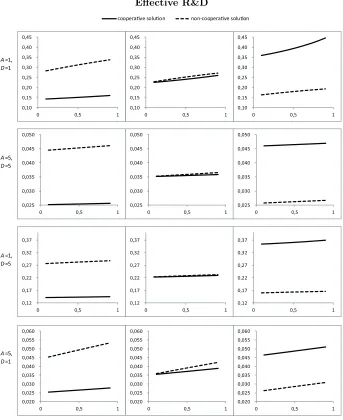
Effective R&D A=1, D=1 A=5, D=5 A=1, D=5 A=5, D=1 0,10 0,15 0,20 0,25 0,30 0,35 0,40 0,45

0 0,5 1

0,10 0,15 0,20 0,25 0,30 0,35 0,40 0,45

0 0,5 1

0,10 0,15 0,20 0,25 0,30 0,35 0,40 0,45

0 0,5 1

0,025 0,030 0,035 0,040 0,045 0,050

0 0,5 1

0,025 0,030 0,035 0,040 0,045 0,050

0 0,5 1

0,025 0,030 0,035 0,040 0,045 0,050

0 0,5 1

0,12 0,17 0,22 0,27 0,32 0,37

0 0,5 1

0,12 0,17 0,22 0,27 0,32 0,37

0 0,5 1

0,12 0,17 0,22 0,27 0,32 0,37

0 0,5 1

0,020 0,025 0,030 0,035 0,040 0,045 0,050 0,055 0,060

0 0,5 1

0,020 0,025 0,030 0,035 0,040 0,045 0,050 0,055 0,060

0 0,5 1

0,020 0,025 0,030 0,035 0,040 0,045 0,050 0,055 0,060

0 0,5 1

coopera!ve solu!on non-coopera!ve solu!on

Figure 4: Impact of parameter values on effective R&D. Vertical axis: total level of R&D (yn_+an_{, y}c_+ac_{), wherea=}x−β

l . Horizontal axis: learning parameter

Firm profits A=1, D=1 A=5, D=5 A=1, D=5 A=5, D=1 0,11 0,12 0,13 0,14 0,15 0,16 0,17 0,18 0,19

0 0,5 1

0,11 0,12 0,13 0,14 0,15 0,16 0,17 0,18 0,19

0 0,5 1

0,11 0,12 0,13 0,14 0,15 0,16 0,17 0,18 0,19

0 0,5 1

0,1122 0,1132 0,1142 0,1152 0,1162 0,1172 0,1182 0,1192 0,1202

0 0,5 1

0,1122 0,1132 0,1142 0,1152 0,1162 0,1172 0,1182 0,1192 0,1202

0 0,5 1

0,1122 0,1132 0,1142 0,1152 0,1162 0,1172 0,1182 0,1192 0,1202

0 0,5 1

0,11 0,12 0,13 0,14 0,15 0,16 0,17 0,18 0,19

0 0,5 1

0,11 0,12 0,13 0,14 0,15 0,16 0,17 0,18 0,19

0 0,5 1

0,11 0,12 0,13 0,14 0,15 0,16 0,17 0,18 0,19

0 0,5 1

0,1122 0,1132 0,1142 0,1152 0,1162 0,1172 0,1182 0,1192 0,1202

0 0,5 1

0,1122 0,1132 0,1142 0,1152 0,1162 0,1172 0,1182 0,1192 0,1202

0 0,5 1

0,1122 0,1132 0,1142 0,1152 0,1162 0,1172 0,1182 0,1192 0,1202

0 0,5 1

coopera ve solu on non-coopera ve solu on

Figure 5: Impact of parameter values on firms profits. Vertical axis: equilibrium profits (Πn_,Πc_{). Horizontal axis: learning parameter (l). Left panel: β = 0.1;}

Consumer’s surplus A=1, D=1 A=5, D=5 A=1, D=5 A=5, D=1 0,25 0,35 0,45 0,55 0,65 0,75

0 0,5 1

0,25 0,35 0,45 0,55 0,65 0,75

0 0,5 1

0,25 0,35 0,45 0,55 0,65 0,75

0 0,5 1

0,234 0,239 0,244 0,249 0,254 0,259 0,264

0 0,5 1

0,234 0,239 0,244 0,249 0,254 0,259 0,264

0 0,5 1

0,234 0,239 0,244 0,249 0,254 0,259 0,264

0 0,5 1

0,25 0,3 0,35 0,4 0,45 0,5 0,55 0,6 0,65

0 0,5 1

0,25 0,3 0,35 0,4 0,45 0,5 0,55 0,6 0,65

0 0,5 1

0,25 0,3 0,35 0,4 0,45 0,5 0,55 0,6 0,65

0 0,5 1

0,234 0,239 0,244 0,249 0,254 0,259 0,264

0 0,5 1

0,234 0,239 0,244 0,249 0,254 0,259 0,264

0 0,5 1

0,234 0,239 0,244 0,249 0,254 0,259 0,264

0 0,5 1

coopera ve solu on non-coopera ve solu on

Figure 6: Impact of parameter values on consumer’s surplus. Vertical axis: equilibrium consumer’s surplus (CSn_{, CS}c_{). Horizontal axis: learning}

Social welfare A=1, D=1 A=5, D=5 A=1, D=5 A=5, D=1 0,55 0,65 0,75 0,85 0,95 1,05

0 0,5 1

0,55 0,65 0,75 0,85 0,95 1,05

0 0,5 1

0,55 0,56 0,57 0,58 0,59 0,6 0,61 0,62

0 0,5 1

0,462 0,472 0,482 0,492 0,502

0 0,5 1

0,462 0,472 0,482 0,492 0,502

0 0,5 1

0,462 0,472 0,482 0,492 0,502

0 0,5 1

0,55 0,65 0,75 0,85 0,95 1,05

0 0,5 1

0,55 0,65 0,75 0,85 0,95 1,05

0 0,5 1

0,55 0,65 0,75 0,85 0,95 1,05

0 0,5 1

0,462 0,467 0,472 0,477 0,482 0,487 0,492 0,497 0,502

0 0,5 1

0,462 0,467 0,472 0,477 0,482 0,487 0,492 0,497 0,502

0 0,5 1

0,462 0,467 0,472 0,477 0,482 0,487 0,492 0,497 0,502

0 0,5 1

coopera ve solu on non-coopera ve solu on

We obtained that varying the learning parameter has almost no impact on innovative R&D, firms’ profits, consumers’ surplus and social welfare. Therefore, even if a higher absorptive parameter increases the efficiency of investing in absorptive research, it has almost no impact on social welfare.

When the free spillover is low, the investment in absorptive R&D, consumers’ surplus and social welfare are higher under non-cooperation than under a RJV. However, cooperation is welfare improving when the free spillover is high.

The investment in innovative R&D is always higher than in absorptive R&D for both the cooperative and non-cooperative cases. This remains true even when the investment cost in innovation is much higher than that of absorp-tion.This is due to the fact that the investment in absorption takes its economic value from innovation.

Increasing the free spillover, leads to higher profits under the two regimes, and to higher social welfare and investments in absorptive research in a RJV. However, increasing the free spillover reduces the investment in absorptive re-search under non-cooperation.

Our model is static, and considers firms that are symmetric in all parameters and results in symmetric non-cooperative and cooperative solutions. Interesting extensions would be to consider asymmetrical firms and a dynamic setting where the stock of knowledge and absorptive capacity evolves over time.

References

[1] D’Aspremont, C., Jacquemin, A.: Cooperative and Noncooperative R&D in Duopoly with Spillovers. The American Economic Review 78, 1133–1137 (1988)

[2] D’Aspremont, C., Jacquemin, A.: Cooperative and Noncooperative R&D in Duopoly with Spillovers: Erratum. The American Economic Review 80, 641–642 (1990)

[3] Suzumura, K.: Cooperative and Noncooperative R&D in an Oligopoly with Spillovers. The American Economic Review 82, 1307–1320 (1992)

[5] Kamien, M.I., Muller, E., Zang, I.: Research Joint Ventures and R&D Cartels. The American Economic Review 82, 1293–1306 (1992)

[6] Amir, R., Wooders, J.: Cooperation vs. Competition in R&D: The Role of Stability of Equilibrium. Journal of Economics 67, 63–73 (1998)

[7] Cohen, W.M., Levinthal, D.A.: Innovation and Learning: The Two Faces of R&D. The Economic Journal 99, 569–596 (1989)

[8] Poyago-Theotoky, J.: A Note on Endogenous Spillovers in a Non-Tournament R&D Duopoly. Review of Industrial Organization 15, 253–262 (1999)

[9] Kamien, M.I., Zang, I.: Meet me Halfway: Research Joint Ventures and Absorptive Capacity. International Journal of Industrial Organization 18, 995–1012 (2000)

[10] Wiethaus, L.: Absorptive Capacity and Connectedness:Why Competing Firms Also Adopt Identical R&D Approaches. International Journal of In-dustrial Organization 23, 467–481 (2005)

[11] Gr¨unfeld, L.A.: Meet me Halfway But don’t Rush: Absorptive Capacity and strategic R&D Investment Revisited. International Journal of Indus-trial Organization 21, 1091–1109 (2003)

[12] Leahy, D., Neary, J.P.: Absorptive Capacity, R&D Spillovers, and Pub-lic PoPub-licy. International Journal of Industrial Organization 25, 1089–1108 (2007)

[13] Kaiser, U.: R&D with Spillovers and Endogenous Absorptive Capacity. Journal of Institutional and Theoretical Economics 158, 286–303 (2002)

[14] Milliou, C.: Endogenous Protection of R&D Investments. Canadian Jour-nal of Economics 42, 184–205 (2009)

[15] Frascatore, M.R.: Absorptive Capacity in R&D Joint Ventures when Basic Research is Costly. Topics in Economic Analysis and Policy 6(1), Article 22 (2006)

[17] Hammerschmidt, A.: No Pain, No Gain: An R&D Model with Endogenous Absorptive Capacity. Journal of Institutional and Theoretical Economics 165, 418–437 (2009)