Computational Studies of Reaction Diffusion Systems by Nonlinear Galerkin Method

Computational Studies of Reaction-Diffusion Systems

by Nonlinear Galerkin Method

Miroslav Kolář

Department of Mathematics, Faculty of Nuclear Sciences and Physical Engineering, Czech Technical University in Prague, Prague, Czech Republic

Email: [email protected]

Received April 2,2013; revised May 1, 2013; accepted May 25, 2013

Copyright © 2013 Miroslav Kolář. This is an open access article distributed under the Creative Commons Attribution License, which permits unrestricted use, distribution, and reproduction in any medium, provided the original work is properly cited.

ABSTRACT

This article deals with the computational study of the nonlinear Galerkin method, which is the extension of commonly known Faedo-Galerkin method. The weak formulation of the method is derived and applied to the particular Scott- Wang-Showalter reaction-diffusion model concerning the problem of combustion of hydrocarbon gases. The proof of convergence of the method based on the method of compactness is introduced. Presented results of numerical simula-tions are composed of the computational study, where the nonlinear Galerkin method and Faedo-Galerkin method are compared for the problem with analytical solution and the numerical results of the Scott-Wang-Showalter model in 1D.

Keywords: Nonlinear Galerkin Method; Scott-Wang-Showalter Model; Compactness Method

1. Introduction

It is well known that many problems often occur when one tries to approximate the complex dynamics of reac-tion-diffusion equations. Especially the error estimate of common methods grows exponentially in time. One pos-sible approach to overcome this problem, known as the Nonlinear Galerkin method is suggested by Marion and Temam in [1]. It is also discussed in [2] and [3]. In this paper we discuss this method and its properties, and ap-ply it to the solution of particular reaction-diffusion model and perform a computational study when the method is compared with the commonly known Faedo-Galerkin method.

Consider a system of reaction-diffusion equations

 

2

2 ,

t x

 _  _

 D F

 

 (1)

where _Dd d,

: d_

F 

 

t x,

denotes a positive definite diagonal

matrix, is a Lipschitz continuous map

and

d



 is a d-dimensional function of time

and space

0

t

 

,

x a b . We consider the homogeneous

Dirichlet boundary conditions  _{x a} _{x b} 0 and the initial conditions

ini

0 .

t 

  (2)

We introduce the space as the

Hilbert space with the scalar product

 



2 _{, ;} d

L a b



H 



 







2_{ ,}

1 1

, , ,

b

d d

i i i i

H L a b i i a

 







        (3)

and the space 1



 



0 , ;

d

H a b



V  as a Hilbert space

endowed with the scalar product









1_{ }

0 ,

1 1

, ,

b

d d

i i x i x i V H a b

i i a

 

  _  _

 



 

 .

      (4)

Let iniH. Then the weak solution of the problem (1)-(2) on time interval



0,T



is a mapping



,T



V

: 0

 such that it satisfies the following equa- tions for each V:



 





 







ini 0

d _{, , , in 0,}

d

.

V t

T t



 



D F

     

 

, (5)

2. Nonlinear Galerkin Method

The nonlinear Galerkin method proposed by Marion and Temam in [1] is an extension of the classical Faedo- Galerkin method, which is extensively discussed in [4], [2] or [3]. Generally there are two main goals we would like to achieve by using the nonlinear Galerkin method:

re-garding the computational time of the Faedo-Galerkin method;

 To decrease computational time regarding to the pre-cision of the approximation of the Faedo-Galerkin method.

Analogically to the Faedo-Galerkin method, we search the approximate solution on some finite-dimensional subspace of . Consider a differential equation for the unknown function

V



2 _{0, ;}

L T

 H



 in the following

form:

 

d

dt   (6)

with the initial condition

 

0  ini,

 

where the mapping  is written as

 

A F

 

    for some linear operator A. The

H is a separable Hilbert space with the orthonormal basis composed of eigenvectors of the op- erator



1 2



, ,

  _

2 xx

 satisfying the homogeneous Dirichlet boundary conditition in

 

a b,

P

.

Then we denote symbols and as projectors

to the subspaces m m

Q



1 2



span ,

P_mH  , _,_m and



Pm





H , respectively. Thus PmH is a finite-dimen-

sional subspace of H generated by first m basis func-

tions and



PmH



 is its orthogonal complement.

Then, the solution 

 

t of Equation (6) can be writ-ten as

 

t pm

 

t qm

 

t ,

 (7) where

 

 

,

 

 

.

m m m m

p t P t q t Q  t

Substituting the decomposition (7) to (6) and applying the operators P_m and Q_m, we get

 



 

 

d _,

d pm t Pm pm t qm t

t   



(8)

 



 

 

d _.

d qm t Qm pm t qm t

t   



(9)

Discretization in the nonlinear Galerkin method is based on the two following steps:

1) Replacing the right hand side by the first order Taylor expansion:



 

 





 







 



 



 

2



,

m m

m m m m

p t q t

p t p t q t q t





  



  

where is the Jacobian matrix of . One suggested approach is that the remainder in the Taylor expansion satisfies these following properties (see [1,2,5]):



 

 



2



d

 

0, 0.

d

m m

q t q t

t

 



This simplification is implied by a particular nonlinear Galerkin method we are using. Then, the second equation of the system (8) can be written as

 







 



 

.

m m m m m

Q  p t  Q  p t q t

2) Replacing the



Pm





H by some finite-dimensional subspace, since we can only operate on some finite- dimensional subspace PMH for Mm instead of the

whole H during the numerical computation. Then the

m

Q H is replaced by



PM Pm



H and instead of func-

tion qmQm

 

t , we consider the function

 



  

.

m M m

z t  P P  t

The equations for the nonlinear Galerkin method can

be finally written as the following:

 



 

 









 









 



 

d _,

d

.

m m m m

M m m M m m m

p t P p t z t t

P P p t P P p t z t

 



   



 

(10)

The degree of approximation is determined by the pa-rameters m and M. We interpret the function as an

approximation of solution of (6) in the space m

p

H and

m as a correction term which modifies for large

values of time t.

z pm

The weak formulation of (10) is obtained easily by multiplicating (10) by basis function j for

1, 2, ,

j _ M . Utilizing the orthogonal projection and

orthonormality of basis functions i, we obtain the weak

formulation of the nonlinear Galerkin method

 





 

 





 













 



 



d _{, ,}

d

, ,

m j m m j

m J m m

p t p t z t

t

p t p t z t

 

J

 

 _{  }

 

 

  



 

(11)

for the indices j1, ,_ m and J m 1, , M . We

endow these equations with the initial conditions

 



pm 0 ,j

 

 Pmini,j



for j1, 2, , . m

3. Application to the Scott-Wang-Showalter

Model

We show the application of the nonlinear Galerkin method on the particular reaction-diffusion system. It was experimentally discovered, that there arise patterns created by flames during the combustion of mixed com-pounds of hydrocarbon gases.

This phenomenon is described by the Sal’nikov model

(see [4,6,7]), which generates the thermokinetic oscilla-tions. The Sal’nikov’s work deals with the problem of the cool flames during the oxidation of hydrocarbon

The scheme of the Sal’nikov’s thermokinetic oscilla-tion is the following:

, h

PA A B eat.

In the first reaction, the compound P generates the

re-active compound A. In the second reaction, the

com-pound A decomposes to the inert product B during the

emergence of heat. The detailed physical point of view is discussed in [6]. The system of reaction-diffusion equa-tions for dimensionless concentration  of reaction intermediate A and dimensionless temperature  of

reaction compounds is:

 

 





2 2

2 2 ,

1 _,

f

x

f Le

x

 _{ } 

 

 

 _{   }

 

  

    

 

(12)

where the function f is defined as

 

exp .

1

f



 

  _ _

 

  (13)

The Le, ,  and the  are the parameters of the

model,  is the dimensionless time. We complement these equation with the initial conditions

ini ini

0 , 0

t t

 _   _   (14)

and with the Dirichlet boundary conditions

, exp

1 ,

x a x b

x a x b



 

  

 

 

 

 

  

   



 (15)

which are the stationary solutions of the (12). We convert the problem (12)-(14) into the homogeneous boundary conditions problem. By subtracting the boundary condi-tions (15) from  and we obtain the system 













2

2

2

2

, exp

1

1

exp 1

f x

f

Le x

  _{ }  _

 





 

  



 

 

 _ _{     }

 

   

  _ 

 

 

  

  

 _{  }

 _       

 

  

   

_{   } 

  



  

(16)

endowed with the homogeneous boundary conditions and with the following initial conditions

ini ini

0 , 0

exp 1

 



  

 

   _{ }    

 _ 

 

 (17)

We consider the unknown functions  and  as mappings from the interval

 

0,T to the V . Denoting

 

,

exp 1

g   

 

 

 

 _ 

 

we introduce the following operator notation for un-

known vector

 

 

 

,,

  





 

 _{ } 

 

 :

 

  



  



 





  







  



2 2

2 2

0

, 1 ,

0 0

0

, 1 ,

0 0

, ,

1

,

1 1

xx xx

xx xx

A C

Le

A C

Le

g f

T R

g f

f g f

Q

f g f





 

 



 

 

  

  

 

 

   _{ }

  _{ }

 

   

  _{ }

 

  _{ }

  _{ }



  

  _{ }

      

   

_{ } 

_ 

   

  _{ }

 



       

 

 _{     } _

 





 





where













2





1 _exp

1 1

f  

 

 

   

    _ _

  

    .

Then we define the operator F as

 

 

F  ACT  R with the Jacobian matrix

 

 

F    A C Q  . Utilizing this notation, we can

rewrite the problem (16)-(17) as

 



 

d _,

d  F  



(18)

ini ini , ini

exp 1



.

 

 

 

 

 

   

   

  _  

 

 

 (19)

In this case, we consider n1,d2, the domain

   

a b,  0,l and the spaces HL2



 

0,l ;2



and

 





0 

1 _{0, ;}

H l



V 2 _{. Let us denote}

 

x 2sin πx

l l

 

  _{ }

 





. For the application of the non-

linear Galerkin method, we use the orthonormal basis of

 1  2 1 0 , . 0           _{ }    _            _  

 (20)

We search the Galerkin approximation of  as the decomposition 

 

  pm

 

 zm

 

 , where the ap-

proximation term pm

 

 and the correction term

 

m

z  are written as

 

 

 

1 1 0 , 0 m m i

m i i

i i i

p    

        _{ }  _{ }     





 

 

 

1 1 0 . 0 M M I

m I I

I m I m I

z    

          _{ }  _{ }     





The unknown combination coefficients  and  for the  1, 2, ,_ M are given by the following system of differential-algebraic equations:

















2 2 2 2 2 2

d π _{, ,}

0 d 0 d π , d 1 1 , , j

j j m m

j j m m

j

j j

j

T p z l

j

Le T p z

l              _  _{ }             _  _         , j    (21)

for j1, ,_ m,

 





 

 

 





 

2 2 2 1 1 2 2 2 1 , , 0 π _, 0 0 0 , , 0 0 1 , , 0 π 1 , 0 J m J M I J

J I m

I m M

J I m

I m I

m J

J

I

J J I m

I m J

T p J Q p l Q p T p J

Le Q p

l                                                          _{     }  _{ }           _                       _{ }         





 

1 0 0 , , M M I m

I m I J

Q p         _{ } _{  }       





(22) for J m 1, ,_ M.

Multiplicating the second equation of (22) by  , using simple algebraic manipulations and subtracting it from the first equation of (22), we obtain a linear relation between _J and _J:

  2 2 2 2 2 2 π π 1 J J C J J l J Le l        (23)

for J m 1,m2, ,_ M . The system (22) for

correc-tion (with dimension 2



Mm



) can be reduced to a

system with the dimension equal to



Mm



for the

unknown coefficients J:

 





 

   

2 2 2 1 1 , , 0 π , 0 0 0 , . 0 J m J M I J

J I m

I m M

J

I m

I m I

T p

J

Q p l

C I Q p

                             _{ }  _{    }                _         







The coefficients J are then computed via the

rela-tion (23).

4. Convergence

We prove the convergence of the nonlinear Galerkin method applied to the Scott-Wang-Showalter model.

The most important note is the existence of the invari-ant region for the Scott-Wang-Showalter model. Its exis-tence was proved in [7].

We introduce the following operator notation

 

 

1 0

, ,

0

D A A Id G A F

Le

 

_{ }     

      ,

where Id is the identical operator. The Jacobian matrix of

the operator G is computed as

 

 

G   A F  Id C Q

 

0

 . Considering the invariant region for the model, the operator G satisfies

the Lipschitz condition with the constant for each

0

 

 and each solution with the initial condition inside te invariant region is bounded, i.e. 

 

x, K,

 

x, K

  for some K0 and for each x

 

0,l

and each 0. Then we have the following estimates for the right hand sides of the model

  



1,

g f K

    

  











2

1 _,

g  f   K

      

where _{1 2} . Hence we can write the following important estimates for the operator :

,

K K 0

G

 

R2 0,

 

R2 R2.

G q k G q u k u₁ (24)

Then the equations for the nonlinear Galerkin method (11) are as follows

 

 





 

 





d

, d_ pm   Apm  P G pm m  zm 

  





 









 



 

.

m M m m

M m m m

Az P P G p

P P G p z

 

 

  



Problem (25) is the system of differential-algebraic equations solvable on



0, m



ue to the theory of ODEs

as the algebraic system for zm is uniqu solvable and

smoothly depends on pm. The value o Tm depends on

quality of approximation.

T d

ely f the

1) Operator A

The operator A has the same eigenfunctions as the

operator A:

 1 _,  2 0 _.

0

 _ _  _{ } _



   



 



The eigenvalues are1  

2

1 ₁ π

l

 

    

 





,

 2 π 2

1 Le l  

   _{ }

 





. The operator A is (see [8]) posi-

tive and self-adjoint. Hence we can define its square root

A as



,





,





,



H _H H

Au v  Au Av  u Av for each

.

 

, Dom

u v A

Now we introduce some useful relations between the operator norms which we use in the next part. For more detailed derivation see [4]

2

2 2 2

2

H H H _H,

Aq  D q  q  D q (26)

2 2 ₂

,

H

H H

Aq  D q  q (27)





2 ₂

min 1, ,

H H

Dq  Le q (28)





2 _{min 1,} 2 2 _.

H H

Dq  Le q (29)

To prove the convergence of the nonlinear Galerkin method we process the particular sequences in Equation (25).

2) Sequence

 

z_{m m}_1

We multiply the second equation of (25) scalarly by

m Az









  





  





, ,

, .

m m H M m m m H M m m m m _H

Az Az P P G p Az

P P G p z Az

 



 

Using the Young inequality, we obtain

 

2

 

2

2 2

2

1 4 1

. 4

m H m _H m H m m _H

m H

Az G p Az G p z

Az



  



According to [1], the expression Az_{m H}2 has its

lower bound

2

2 min

1

m H m m _H Az   _ Az

and then we can write

 

 





2 2 2

min

1 2 .

m m m _H m m _H

H

Az G p G p z

 

  

Using estimates (24), we obtain











2

2 0 1

2 2 2

.

1 min 1, 1 π

m H m

H

k k z Az

Le m

 

 

We use relations (27) and (28) on the left hand side of this inequality. Then we obtain the estimate for zm

via the Poincaré inequality:



















2

2 2

0 1

2

2 2 2

2min 1, 1 .

1 min 1, 1 π

m H m H

k k z

Le z

Le m



 

 

Hence z_{m H}2 0 for m uniformly on the

in-terval

 



0,



.

3) Sequence

 

p_{m m}_1

,

A A a Id are linear operators. We suppose that

ini-tial condition 0Dom

 

A Dom



A



. Using the Bessel inequality, we obtain following auxiliary esti-mates

 

 

 

ini ini

ini ini

ini ini

0 ,

0 ,

0 .

m H m H H

m m

H H

m H m H H

p P

A p AP A

Ap AP A

 

 

 

 

 

 

H (30)

We multiply the first equation of (25) scalarly by

m Ap













d , d

, ,

m m H

m m H m m m m H. p Ap

t

Ap Ap P G p z Ap

 

 

 

   

Using the definition of the square root of operator A,

we obtain









2 ₂

d _{, .}

d m H m H m m m m H

A p Ap P G p z Ap

t   

We use the Young inequality and (24) to estimate the left hand side and then we obtain the auxiliary estimate

2 ₂

2 0

d _.

d_t A pm _H Apm Hk (31) 4) Boundedness of



Ap_{m m}



_1 in _L2



_{0, ;T H}



We integrate the Equation (31) over

 

0,T :

 

2

 

2 ₂

0

0 0

d .

T T

m m _H

H

A p  Ap  

 _{  }

 

 



k T

Dropping the m

 

2 H

A p T and using(30) we obtain

 

2 ₂ 2

0 in

0

d .

T

m _H i

H

Ap   k T A





1_{Denoting the }max _{the largest one and the the smallest one.}



min

Hence the sequence



Apm



_m1



 is bounded in



2 _{0, ;}

L T H



for each T0.



Ap





5) Boundedness of _{m m1} in L



0, ;T H



We integrate the Equation (31) over

 

0,T :

 

2

 

2 ₂

0

0 ₀

d .

T T

m m _H

H

A p  Ap  

 _{  }

 

 



k T

Dropping the integral of nonnegative function and using (30) we obtain

 

2 2

2

0 in .

m i

H H

A p T k T A

Hence the sequence





1

m m A p



 is bounded in



0, ;

L T H



for each T 0.

6) Boundedness of









1 0, ;

m _m

A p  L H

 

Using the relations (26) and (27) we get the inequality

2 2

.

H _H

Aq  Aq

The auxiliary relation (31) then leads to

2 2

2 0

d _.

d m m

H H

A p A p

  k

Using the Grönwall lemma for

 

m

 

2 H y   A p  ,

and

1

k Ak₀2 we obtain

 

2 2





2

ini 0

e e

m

H H

A p   _ A k  _

  1 .

Hence the sequence





1

m m A p 

 is bounded in



0, ;



L  H .

7) Sequence  

  1

d d m

m

p



 

We multiply the first equation of (25) scalarly by

d d_ pm:





d d

,

d d

d

, , d

d d

m m

H

m m m m m .

H H

p p

Ap p G p z p

 

 

 

 

 

   

 _{ } _  _

   

We use the Young inequality for 1 on the last term and estimate the middle term.





2

2 2

1 d 1 d 1 _.

2 d m 2 d m 2 m m _H

H H

p A p G p z

    

Using the boundedness of the operator G (24) we

obtain

2

2 2 0

d d

.

d m d m

H H

p A p

   

We integrate this inequality over

 

0,T and use the

relations (30):

 

2 2 ₂ 2

0 0

d

d .

d

T

m m

H H

H

p   A p k T

   



A

Hence the sequence

1

d

d m

m p

 



 

 

  is bounded in





2 _{0, ;}

L T H .

9) Passage to the limit

Considering the previous estimates (boundedness of

m

A p and (27) particularly), we obtain the following

properties

 













1

1

is bounded in 0, ; ,

is bounded in 0, ; ,

m m x m m

p L

p L

 



 _





 

H

 H

whereas













2



0, ; 0, ; ,

0, ; 0, ; .

L L T

L L

 



 

  

H H



H H

Hence the sequence

 

p_{m m}_1 is bounded in L2



0, ;TV



0

 . This m that we can choose a subse-quence

 

pm m₁



for each T eans



  , which converges weakly in





2 _{0, ;}

L TV .

Using the Aubi a (see [9]) fo

fu

,

n Lemm r following

nction spaces:

0 , , 1

X V X H X H

we obtain that the Banach space









2 _{0, ;} d 2 _{0, ;}

d

T

W L T L T



 

_   _

 V  H 

with norm

 

 

2

2

0, ,

0, ,

d d

T

W L T

L T



 _V 

H

  

is compactly embedded in 2



_{0, ;}



L T H .



is boun Since the sequence

 

p_{m 1} ded

m in





2

k

0, ;

L T V and sequence

1

d 

d m

m p

 



 

  is bounded in





2 _{0, ;}

L T H for each T 0, there exists a subsequence

 

k ₁ k

m _m p 

 , which converges strongly to the limit point p





2 _{0, ;}

L T H . Knowing that the sequence

 

p 

in m m₁

converges weakly in 2



_{0, ;}



L T V , we obtai

uniqueness of the limit th , ;T V



. 10) Sequence



G p



z

n from

at 2 ₀

pL









1

m m _m

Since the operator satisfies the Lipschitz condition, w

G





 

_{ }



 



 



 

 

 

     



2 2

2 2



0, ; 2 0 2 2 0 2 2 0, ; 2 2 2 2

0, ; 0, ;

d

d

0.

L T T

m m _H

T

m m _H

m m L T

m L T m L T

G p z G p

p z t p

p z p

p p z

2

m m

G p z G p

                  





H H H H   

Hence strongly in

 



m m



 

G p z G p L2



0, ;T H



.

11) Existence ak solution

rt nd uniqueness of

and uniqueness of we

In this pa we prove the existence a th

Th

e weak solution of the Scott-Wang-Showalter model. e existence is proven via the strong convergence of the sequence



G p



m zm





_m1

 

 .

We multiply the first equation of (25) by j for

1, ,

j _ m .













d d , , , . m j H

m j _H m m j _H

p

Ap G p z

              

Multiplying the previous relation by the test function and integrating it over 

 





1 _0,

C T

  , 

 

T 0

 

0,T

we obtain

 

 

 

 









 

 





 

0 0 d , d d , d

, d .

T

m j H T

m m j _H

T

m j

H

p t

G p z

A p A

   0                  _  _    _{ }





   

Integrating the left hand side per parts and passing to the limit we obtain

    







 



 



 

 











 



 

ini d , 0 T j _H   0 0 , d d

, , d .

j _H T

j j

H H

p

G p A p A

                 _  _





(32) Additionally, we consider . Then

 





0 0, C T _ 



,





,





,

d j





j



d

j

H H

p A p A 

   H G p

 (33)

in sense of distributions.

Now, we multiply the Equation (33) by 1



_0,



C T

  ,

 

T 0

  and integrate it over

 

0,T . Using integration

per parts we obtain

 





 



 



 

 











 



 

0 d 0 , d T

j _H j _H

T

    



0

0 , d

, j _H , j d .

H

p p

G p A p A

            

_

_  _ (34)

Subtracting (32) and (34) we get 

_

 



p 0 0,j



_H 0 for eachj,

which means that p

 

0 ₀. Hence is the weak

solution.

To show the uniqueness, we suppose th e are two ons

p

er different weak soluti  and , which satisfy











 











d , , , , d

 





 

 

ini

d _{, , , ,}

d

0 0 .

j _H j j _H

H

A A G

A A G

              

j _H j j _H

H

 

 

  

  

We denote   

, multiply it by

. Then we subtract the previ-ous equations



,j



_H and sum it over

1, 2,

j _.



 











 

 









, , , , .

j _H j H j

j _H j

d _{, ,}

d j _H j _H

j H j A A G G       





     Hence   



 

 

 





2 2 1 d , .

2 d  H  A H  G  G   H

Finally, using the Young inequality for the last term and Lipschitz condition of operator G, we obtain





2 2

d 2 _{1 .}

d  H     H

Choosing _y

 

_

 

_ 2 _,k



2 ₁



H

      and A0,

we use the Grönwall lemma:









 

2

2 2

0

exp 1 0 0.

H  H



  



  

Hence 

 

t 0 for each 0, which is the con-

tradiction.

5.

titative

er we deal with the error measurement and nlinear Galerkin method diffusion model. We are

Quan

Analysis

In this pap

computational time of the no aplied to a particular

the function subspace, where the approximation of the solutions is searched. Before the application on the Scott- Wang-Showalter model, we use the single one-dimen- sional reaction-diffusion equation with the known ana-lytical solution uu t x

 

, as a benchmark for the

method. Consider the equation

method. The linear systems for correction are solved via Gauss elimination method since they are generally a sys-tems with dense matrices.

We plot the norm of the difference between ana-lytical solution and numerical approximation, i.e.

2 L

2

analytical numerical _L

u u in specific time intervals. Time is

measured in seconds. Additionally, Table 1 of computa-tional complexity is included.

 

 

2

2 ,

u u

f u g t x t x

 

  

 (35)

for x

 

0,1 and tt_ini satis



fying the homogeneous

Dirichlet boundary condition and initial condition 5.1. Simulation 1 Consider equation





ini ini, ,

t t

u _ u t x

re f is a ar fu

that u

is the analytical so of the pro simulations we u er

(36)

 

2 2

2 2 ,

u u

u g t x

t x

 

  

 

whe nonline nction of u and g is a chosen

function of time ttini and space x

 

0,1 , such with initial condition _u sinπ_xsin

 

_t ini

t t and with

the analytical solution u in form

ini

 

, sinπ sin

u t x  x t.

The time evolution of error is on the Figures 1 and 2. lution

se eith

blem (35)-(36). In all

10

m , M 0 (which is the

case of the commonly known Faedo-Galerkin method- see [4]) or m 5 in the Galerkin

approxima-tion.

The explicit form of n

5, M _{Table 1. Computational complexities for testing}

simula-tions.

 

,

g t x

functio for all dis-cussed cases, equations for the nonlinear Galerkin ap-proximation d scalar products can be eas-ily de

Simulation Faedo-Galerkin _method Nonlinear Galerkin _method

Simulation 1 1307.71 s 322.03 s

Simulation 2 8345.08 s 1910.25 s

Simulation 3 6269.52 s 2161.48 s

and enumerate rived or found in [4].

ial equ

The systems of ordinary different ations for ap-proximation from the nonlinear Galerkin method are solved by means of time-adaptive Runge-Kutta-Merson

[image:8.595.61.538.354.553.2]

(a) (b) (c)

Figure 1. Time evolution of errors for the Faedo-Galerkin method. (a) Simulation 1; (b) Simulation 2; (c) Simulation 3.

[image:8.595.68.535.576.718.2]

(a) (b) (c)

5.2. Simulation 2

Consider equation

 

2

3

2 ,

u u

u u g t x t x

 _ _{  }

 





 

ini sinπ sin 2π sin ini

t t

u _  x x 

lution equals to

with initial condition t

and with analytical so

  

, sinπ sin 2π



sin

u t x  x x  t

error is on the Figures 1 and 2.

. The time evolution of

5.3. Simulation 3

Consider equation

 

2

3

2 ,

u u

u u g t x t x

 _ _

   

with initial condition



sin 5πx



sin sin 2





tini





error is on the Figures 1 and 2.

tudies

In this section we present the computational results for the Scott-Wang-Showalter model. Cons ering the

ho-dition problem (16)-(17), we ur of the model depending on various initial conditions and various sets of par eters. Additionally, deeper computational study can be found in ime evolution of function

boundary condition problem nitial conditions

ini sinπ

t t

u _  x

and with analytical solution equals to

  

, sinπ sin 5π



sin sin 2



 



u t x  x x  t .

The time evolution of

6. Qualitative S

id mogeneous boundary con

investigate the behavio

am

[4]. The following figures show the t

.

6.1. Simulation 4

We solve the homogeneous (16)-(17) with the following i

 2

50 2.5 ini 0, ini e

x

 _{  }  

(37) for x

 

0,5 ,0. The parameters of the model are

1.8, 0.0005,Le 1, 0.18

    and the number of

modes in the Galerkin approximation is mM 60.

The time evolution of the problem is on the Figure 3.

6.2. Simulation 5

eneous boundary condition problem initial conditions

(38) We solve the homog

(16)-(17) with the following

 2

50 1.25

e , < 2.5,

0,

x x



 



    _{ }2

ini ini

50 3.75

e x ,

x

 

 2.5

for x

 

0,5 ,0. The parameters of the model are

(a)

(b)

[image:9.595.313.537.83.604.2]

(c)

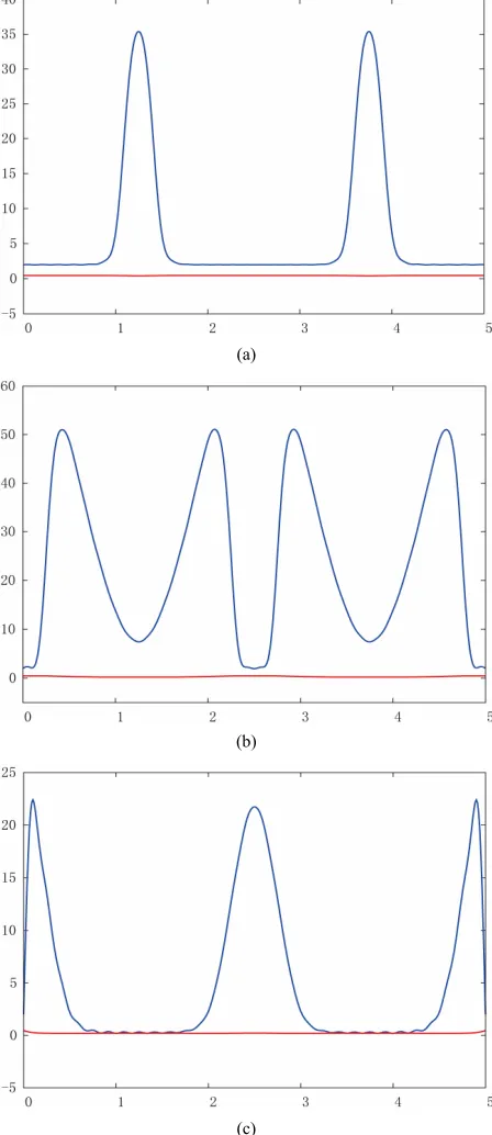
Figure 3. Simulation 4—time evolution of the functions Θ

(blue line) and α (red line). (a) τ = 0.00614; (b) τ= 0.01814; (c) τ= 0.02214.

2, 0.0005,Le 2.6, 0.18

    

modes in the Galerkin approximat

and the number of ion is mM 60.

The time evolution of the problem is on the Figure 4.

7. Conclusion

(a)

(b)

[image:10.595.60.284.89.606.2]

(c)

Figure 4. Simulation 5—time evolution of the functions (blue line) and α (red line). (a) τ = 0.00511; (b) τ = 0.01311; (c) τ = 0.02025.

the particular system of reaction-diffusion equations in one spatial dimension. As the investigated reaction-dif-fusion system was chosen the Scott-Wang-Showalter model. We presented the system of differential-algebraic

equations for the approximation of the weak solution, proof of existence and uniqueness of the weak solution and the proof of convergence of the nonlinear Galerkin method. We performed quantitative analysis among ana-lytical solution and numerical approximations obtained via the nonlinear Galerkin method and the commonly known Faedo-Galerkin method. It indicates that the non- linear Galerkin method is more efficient since it con-serves the similar level of accuracy with respect to the shorter computational time.

8. Acknowledgements

Partial support of the project No. TA0102871 of th Technological Agency o e Czech Republic, No.

outh and Sport of the Czech Republic is

Θ

e f th

SGS11/161/OHK4/3T/14 of the Czech Technical Uni-versity in Prague, No. MSM 6840770010 of the Ministry of Education, Y

acknowledged.

REFERENCES

[1] M. Marion and R. Temam, “Nonlinear Galerkin Meth-ods,” SIAM Journal on Numerical Analysis, Vol. 26, No. 5, 1989, pp. 1139-1157. doi:10.1137/0726063

[2] J. Šembera and M. Beneš, “Nonlinear Galerkin Method for Reaction-Diffusion Systems Admitting Invariant Re-gions,” Journal of Computational and Applied Mathe-matics, Vol. 136, No. 1-2, 2001, pp. 163-176.

doi:10.1016/S0377-0427(00)00582-3

[3] J. Mach, “Application of the Nonlinear Galerkin FEM Method to the Solution of the Reaction Diffusion Equa-tions,” Journal of Math-for-Industry, Vol. 3, 2011, pp.

41-51.

[4] M. Kolář, “Mathematical M lations of Reaction-Diffusi

odelling and Numerical Simu-on Processes,” Diploma Thesis, Department of Mathematics FNSPE CTU, Prague, 2012. [5] A. Debussche and M. Marion, “On the Construction of

Families of Approximate Inertial Manifolds,” Journal of Differential Equations, Vol. 100, No. 1, 1992, pp. 173- 201. doi:10.1016/0022-0396(92)90131-6

[6] S. K. Scott, J. Wang and K. Showalter, “Modelling Stud-ies of Spiral Waves and Target Patterns in Premixed Flames,” Journal of the Chemical Society, Faraday

Trans-actions, Vol. 9 -1739.

doi:10.1039/a6

3, No. 9, 1997, pp. 1733

08474e

[7] V. Tomica, “Reaction-Diffusion Equations in Combus-tion,” Proceedings of Czech Japanese Seminar in Applied Mathematics, Prague, 30 August-4 September 2010, pp.

n des Pro- 84-93.

[8] R. Temam, “Infinite-Dimensional Dynamical Systems in Mechanics and Physics,” Springer, Berlin, 1997.