Munich Personal RePEc Archive
Environmental Kuznets curve in
Indonesia, the role of energy
consumption and foreign trade
Saboori, Behnaz and Soleymani, Abdorreza
School of Social Sciences, Universiti Sains Malaysia,
14 June 2011
1
ENVIRONMENTAL KUZNETS CURVE IN INDONESIA, THE ROLE OF ENERGY
CONSUMPTION AND FOREIGN TRADE
Behnaz Saboori*, Abdorreza Soleymani
School of Social Sciences, Universiti Sains Malaysia, 11800 Penang, Malaysia
*
Corresponding author: B. Saboori, School of Social Sciences, Universiti Sains Malaysia, 11800
Penang, Malaysia. Email: behnazsaboori@yahoo.com Tel: +60176168939
Abstract
This study examines the dynamic relationship among carbon dioxide (CO2) emissions, economic
growth, energy consumption and foreign trade based on the environmental Kuznets curve (EKC)
hypothesis for Indonesia during the period 1971–2007. The Auto regressive distributed lag
(ARDL) methodology is used as an estimation technique. The results do not support the EKC
hypothesis, which assumes an inverted U-shaped relationship between income and
environmental degradation. The long-run results indicate that foreign trade is the most significant
variable in explaining CO2 emissions in Indonesia followed by Energy consumption and
economic growth. The stability of the variables in estimated models is also examined. The result
suggests that the estimated models are stable over the sample period.
Keywords: Environmental Kuznets curve, CO2 emissions, energy consumption
2
1. Introduction
Global environmental issues are getting more attention especially the increasing threat of global
warming and climate change. Higher global average air and ocean temperatures, widespread
melting of snow and ice, and rising global average sea level are some evidence of warming of the
climate system. The intergovernmental panel on climate change (IPCC) reported a 1.1 to 6.4 °C
increase of the global temperatures and a rise in the sea level of about 16.5 to 53.8 cm by 2100
(IPCC, 2007). CO2 emissions which is a global pollutant is the main greenhouse gas that causes
58.8% of global warming and climate change (The World Bank, 2007a). Rapid increase of CO2
emissions is mainly the result of human activities due to the development and industrialization
over the last decades.
In this subject one strand of literature focuses on testing the growth and environmental pollution
nexus that tests the environmental Kuznets curve (EKC) hypothesis which proposes a U-type
relationship between environmental quality and economic growth. They tried to answer the
question whether continued increase in economic growth will eventually undo the environmental
impact of the early stages of economic development. Many related studies are available in Stern
(2004) and Dinda (2004). More recent examples are those of Dinda and Coondoo (2006),
Akbostanci et al. (2009), Lee and Lee (2009), Fodha and Zaghdoud (2010) and Narayan and
Narayan (2010). Their results differ substantially and are inconclusive.
As one of the crucial elements for continuous economic growth is energy consumption, the
second strand of the literatures is related to energy consumption and output nexus. Several
studies emerged in this regard. After the pioneer seminal study of Kraft and Kraft (1978) who
found a unidirectional Granger causality running from output to energy consumption for the
3
countries, Masih and Masih (1996), Yang (2000), Wolde-Rufael (2006) and Narayan et al.
(2008) tested the energy consumption and economic growth nexus and found varied and
sometimes conflicting results. With the development of time series econometric techniques
Masih and Masih (1997), Cheng and Lai (1997), Al-Iriani (2006), Mehrara (2007), Akinlo
(2008), Ghosh (2009), Tang (2008), Chandran et al. (2009) and Yoo and Kwak (2010) focused
on the cointegrating relationship between output and energy consumption.
Two important points come to light from reviewing these two groups: First, as most of them
consider the growth–environment nexus and growth–energy nexus in a bivariate framework,
thus, suffer from omitted variables bias, hence making a study of both nexuses in a single
framework is necessary. Second, as the vast majority of these investigations concentrate on using
the cross-country panel data, therefore they would not allow the impact of environmental
policies, historic experiences, development of trade relationship and other exogenous factors
through time to be examined. However, a time series analysis for a single country may provide
better framework to estimate these relationships. Therefore, studying countries individually may
be necessary.
The third strand filled the gap in literature by combining these two lines of studies and
examining the dynamic relationship between carbon emissions, energy consumption and
economic growth in a single framework for single countries. See for example, Ang (2007, 2008),
Soytas and Sari (2009), Zhang and Cheng (2009), and Ghosh (2010).
In a similar kind of study Halicioglu (2009) for Turkey, Jalil and Mahmud (2009) for China and
Iwata et al. (2010) for France attempted to reduce the problem of omitted variable bias in
4
In this regard, they applied ARDL approach of cointegration in a log-linear quadratic equation
among CO2 emissions, energy consumption, economic growth and trade openness to test the
validity of EKC hypothesis. Halicioglu (2009) found two forms of long-run relationships
between variables when CO2 emissions and income are the dependent variables. He suggested
that the most significant variable in explaining the carbon emissions in Turkey is income
followed by energy consumption and foreign trade. Jalil and Mahmud (2009) found a
unidirectional causality running from economic growth to CO2 emissions in China. The results of
the study also indicate that the carbon emissions are mainly determined by income and energy
consumption in the long run. Moreover trade has a positive but statistically insignificant impact
on CO2 emissions. Iwata et al. (2010) as well as the two previous studies supported the EKC
hypothesis in the case of France. They found evidence of statistical significance for the
coefficient of energy consumption just in the short run. Furthermore they concluded that foreign
trade coefficient is not statistically significant in the short and long run.
This paper is an attempt to extend the literature by considering the long-run relationship between
CO2 emissions, economic growth energy consumption and foreign trade for Indonesia based on
the EKC hypothesis. The issue of environmental pollutants is in a progressive trend in
developing countries as they require more energy consumption for higher economic
development. Consequently, they suffer from more environmental problems. Among the
developing countries, Indonesia has been one of the fastest-growing open country with a rapid
economic transformation, population expansion and high energy consumption with particular
emphasis on city context and a significant rise in pollutant emissions, specifically CO2
5
trend of global warming continues unabated, it is expected that 2000 of the 17000 islands in
Indonesia will be submerged by 2030 (Lean & Smyth, 2010).
The choice of this country is also motivated by the fact that no known study has been conducted
to examine the dynamic relationship between CO2 emissions, economic growth, energy
consumption and trade openness in a single framework for Indonesia.
Our investigation is based on environmental Kuznets curve hypothesis, using time series data
and coitegration analysis. To conduct cointegration analysis we employ the recently developed
ARDL bounds testing approach of cointegration by Pesaran and Shin (1999) and Pesaran et al.
(2001). The main objective of the current study is examining the long-run relationship amongst
CO2 emissions, economic growth, energy consumption and trade openness in Indonesia during
the period 1971-2007.
The rest of the paper is structured as follows: In section 2 the model and econometrics
methodology are introduced while section 3 is data and section 4 gives the empirical results and
the last part is the conclusion.
2. Model and Econometric Methodology
Based on EKC hypothesis, it is possible to form a linear quadratic relationship between
economic growth and environmental degradation. However to eliminate the omitted variable bias
Dina (2004) proposes other variables such as international trade, demography, technological
progress and energy consumption as the determinant of environmental pollution. Based on this
argument we take into account the effects of energy consumption and trade openness on CO2
6
between CO2 emissions, economic growth and energy consumption for our baseline estimation
model in logarithm version as follows:
t t t
t
t Y Y EN
E ln (ln ) ln
ln 0 1 2 2 3 (1)
Where E is per capita CO2 emissions, Y represents per capita real income, EN stands for
commercial energy use per capita and is the standard error term. Based on EKC hypothesis the
sign of is expected to be positive whereas a negative sign is expected for . Since higher
level of energy consumption leads to greater economic activity and stimulates CO2 emissions,
is expected to be positive.
To date, various methods have been developed and introduced to conduct cointegration analysis,
such as the residual-based approach proposed by Engle and Granger (1987), the maximum
likelihood-based approach proposed by Johansen and Juselius (1990), the fully modified OLS
procedures of Phillips and Hansen’s (1990) and the recently developed approach, autoregressive
distributed lag (ARDL) by Pesaran et al. (2001). ARDL for cointegration analysis has a number
of attractive features over other alternatives (Pesaran & Shin, 1999). The main advantage of
ARDL approach is that, it does not require establishing the order of integration of the variables.
In this study ARDL bounds testing approach is employed to examine the long-run relationship
among CO2 emissions, economic growth and energy consumption. ARDL framework of Eq. (1)
of the baseline estimation model is as follows:
t t t t t n k n k n k n k k t k k t k k t k k t k t EN Y Y E EN Y Y E E
1 4 2 1 3 1 2 1 11 1 1 1
4 2 3 2 1 0 ln ) ln( ln ln ln ) (ln ln ln ln (2)
In the ARDL bounds testing approach the first step is to estimate Eq. (2) by ordinary least square
(OLS) method. The null hypothesis of no cointegration or no long-run relationship, H0: =
7
conducted to test the presence of long-run relationship among the variables. The critical values
of the F-statistics in this test are available in Pesaran and Pesaran (1997) and Pesaran et al.
(2001).1 Two sets of critical values are found for a given significance level, with and without a
time trend, one for I(0) variables and the other set for I(1), which are known as lower bounds
(LCB) and upper bounds critical values (UCB) respectively. This provides a band covering all
possible classifications of the variables into I(0) and I(1). If the computed F-statistic is higher
than the UCB, the null hypothesis of no cointegration is rejected and if it is below the LCB the
null hypothesis cannot be rejected, and if it lies between the LCB and UCB the result is
inconclusive. At this stage of the estimation process the optimum lag orders of the variables can
be selected on the basis of Schawrtz–Bayesian criteria (SBC) and Akaike’ s information criteria
(AIC). The SBC selects the smallest possible lag length, while AIC is employed for selecting the
maximum relevant lag length. The long-run relationship among variables can be estimated after
the selection of the ARDL model by AIC or SBC criterion, Once a long-run relationship has
been established, error correction model (ECM) can be estimated.
The error correction term (ECT) indicates the speed of the adjustment and shows how quickly
the variables return to the long-run equilibrium and it should have a statistically significant
coefficient with a negative sign. Moreover Pesaran et al. (1999, 2001) suggested testing the
stability of estimated coefficients through cumulative sum (CUSUM) and cumulative sum of
squares (CUSUMSQ). In this study the stability tests such as CUSUM and CUSUMSQ are
conducted to check the stability of the coefficient in estimated models.
Furthermore, following Jalil and Mahmud (2009) and Iwata et al. (2010), in order to avoid the
omitted variable bias, we expand the baseline equation 1 to incorporate trade openness which
may have effect on CO2 emissions. The expected sign of the coefficient of trade is mixed
1
8
depending on a level of a country in economic development stages. It is expected to be negative
for developed countries as they specialize in clean and service intensive production and instead
they import the pollution-intensive products from other countries with less restrictive
environmental protection laws. On the other hand it may be positive in the case of developing
countries as they are likely to be net exporter of pollution-intensive goods (Grossman & Krueger,
1995).
3. Data
The current study uses the annual data spanning from 1971 to 2007 which is based on the
availability of all data. For estimation, Per capita carbon dioxide (CO2) emissions, per capita
GDP, commercial energy consumption per capita and trade ratio were used. All data were
collected from World Bank’s World Development Indicators (WDI) online database. CO2
emissions (E) is measured in metric tones per capita, the real per capita GDP (Y) is in constant
2000 USD, energy consumption (EN) is measured as kg of oil equivalent per capita and trade
openness ratio (TR) is the total value of real import and real export as a percentage of real GDP.
4. Empirical Results
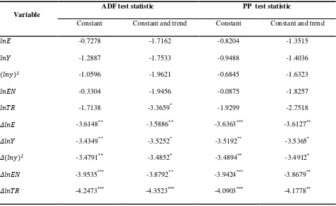
The preliminary step in this analysis is concerned with establishing the order of integration of
each variable as the bounds testing approach is applicable for variables that are I (0) or I (1). The
analysis begins by investigating the unit root test of variables using the augmented Dickey–
Fuller (1979) ADF and Phillips-Perron (1988) PP tests. In both tests the null hypotheses of the
series has a unit root is tested against the alternative of stationarity. Table 1 summarizes the
9
differences of the variables. The results suggest that all the series are stationary in their first
differences, indicating that they are integrated at order one, hence validate the use of bounds
[image:10.612.72.545.181.471.2]testing for cointegration.
Table 1: Unit root tests.
Variable
ADF test statistic PP test statistic
Constant Constant and trend Constant Constant and trend
-0.7278 -1.7162 -0.8204 -1.3515
-1.2887 -1.7533 -0.9488 -1.4036
-1.0596 -1.9621 -0.6845 -1.6323
-0.3304 -1.9456 -0.0875 -1.8257
-1.7138 -3.3659* -1.9299 -2.7518
-3.6148** -3.5886** -3.6363*** -3.6127**
-3.4349** -3.5252* -3.5192** -3.5365*
-3.4791** -3.4852* -3.4894** -3.4912*
-3.9535*** -3.8792** -3.9424*** -3.8679**
-4.2473*** -4.3523*** -4.0903*** -4.1778**
Note: 1. ***, ** and * are 1%, 5% and10% of significant levels, respectively. 2. The lag length has been chosen based on the AIC for ADF test
and the bandwidth is selected using the Newey–West method for PP test.3. The maximum number of lags is set to be four.
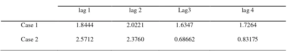
We then proceeded with F-test to confirm the existence of the cointegration between variables.
To follow the procedure of ARDL bounds test we set different orders of lags for the variables as
evidence of previous researches reveals that the results of the F-test are sensitive to the lag
imposed on each of the first differenced variable (Bahmani-Oskooee & Brooks, 1999). We
confirm this by imposing up to four lags on all first differenced variables.2 The results of
2
10
baseline equation (2) are presented as case 1, whereas the results of the case in which baseline
equation (2) is expanded to incorporate trade are provided as case 2. The results are as reported
[image:11.612.65.524.225.307.2]in Table 2 along with the critical values at the bottom of the Table.
Table 2: The results of F-test for cointegration.
Calculated F-statistics for different lag lengths
lag 1 lag 2 Lag3 lag 4
Case 1 1.8444 2.0221 1.6347 1.7264
Case 2 2.5712 2.3760 0.68662 0.83175
Note: 1. 1% CV [3.817, 5.122], 5% CV [2.850, 4.049] and 10% CV [2.425, 3.574] for Case 1.
2. 1% CV [3.516, 4.781], 5% CV [2.649, 3.805] and 10% CV [2.262, 3.367] for Cases 2.
3.The critical values are obtained from Table CI in Pesaran et al. (2001, p. 300).
The results confirmed that F-test is sensitive to the lag lengths. The calculated F-statistics
indicate that there is no cointegration relationship in both cases. The evidence of no cointegration
in cases 1 and 2 is attributed to the fact that the same number of lags were imposed on each
first-differenced variable arbitrarily (Bahmani-Oskooee & Kantipong, 2001).
At this stage, the optimum number of lags on the first differenced variables is usually obtained
from unrestricted vector auto regression (VAR) by means of AIC and SBC. Given the number of
variables and sample size in this study, we conduct optimal lag selection by setting the maximum
lag lengths up to 2. Setting 2 as the maximum lag length helps to ensure that the degree of
freedom is sufficient for econometric analysis. AIC has been used to find the optimum number of
lags in the model. Given this, the AIC-based ARDL suggests ARDL(2,1,2,1) for the case 1 and
11
To further justify our result, we carried out the bounds test after imposing the optimum lags on
each of the first differenced variable. In case 1, the F-statistics of 1.44 was obtained which is still
lower than the lower bound critical value of 2.425 at 10% significant level and does not support
cointegration. In the case 2 the F-statisticsis 6.03 which is higher than the upper bound critical
value of 4.781 at 1% significant level and supports cointegration. The coefficient of ECM (-1) is
correctly signed and statistically significant at 1% significance level in both cases. Following
Kremers et al. (1992) who argued that the significant lagged error-correction term is a more
efficient way of establishing cointegration, we conclude the existence of a strong cointegration
relationship among variables in both cases.
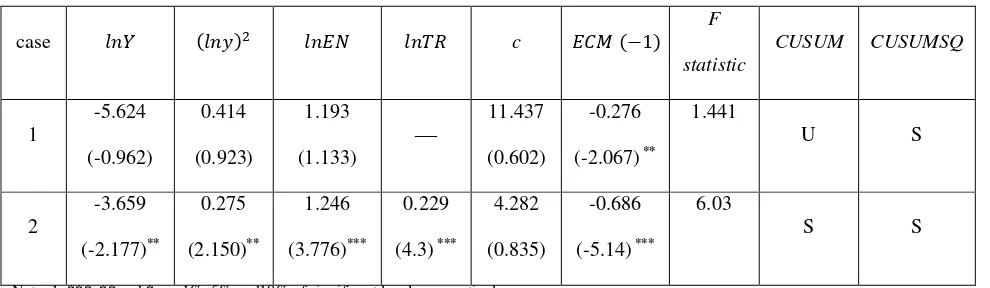
The existence of cointegration among variables warrants the estimation of baseline equation (2)
and the expanded equation by ARDL cointegration approach to get the long-run coefficients. The
[image:12.612.66.561.428.572.2]results are reported in Table 3.
Table 3: estimation results using ARDL approach.
case c
F
statistic
CUSUM CUSUMSQ
1 -5.624 (-0.962) 0.414 (0.923) 1.193 (1.133) 11.437 (0.602) -0.276
(-2.067) **
1.441
U S
2 -3.659 (-2.177)** 0.275 (2.150)** 1.246 (3.776)*** 0.229
(4.3) ***
4.282
(0.835)
-0.686
(-5.14) ***
6.03
S S
Note: 1. ***, ** and * are 1%, 5% and10% of significant levels, respectively
2. ‘‘S’’ and ‘‘U’’ stand for stable and unstable respectively.
12
The negative and positive coefficient of and respectively, in both cases, indicate the
existence of a U-shape relationship between per capita CO2 emissions and per capita real GDP.
Thus confirms that CO2 emissions declines at initial level of economic growth then reaches a
turning point and increases with the higher level of economic growth.
The long-run elasticity of CO2 emissions with respect to energy consumption is positive in both
cases. It is significant at 1% level in case 2, while it is not statistically significant in case 1. This
positive effect of per capita energy consumption on CO2 emissions is in line with Jalil and
Mahmud (2009) and Ang (2008). The coefficient of is 0.229 which is positive in sign and
highly significant. This is in line with Halicioglu (2009). It indicates that 1% increase in foreign
trade will lead to 0.229% increases in per capita CO2 emissions. The positive long-run
relationship between CO2 emissions and trade openness is in line with Iwat et al. (2010).
Insignificant coefficients in case 1 may be attributed to the omitted variable bias. So as can be
seen from the results in Table 3, in case 2 it has been solved with the inclusion of trade variable.
To check the stability of the coefficients cumulative sum (CUSUM) and cumulative sum of
squares (CUSUMSQ) techniques were employed. Graphically, these two statistics are plotted
within two straight lines bounded by the 5% significance level. If any point lies beyond this 5%
level, the null hypothesis of stable parameters is rejected. While the result of CUSUMSQ test
supports the stability of all the estimated variables in both cases, there are some signs of
instability based on CUSUM test in case 1.
5. Conclusion
This paper investigated the long-run relationship between carbon dioxide emissions, economic
13
1971–2007. Furthermore we expanded the baseline equation by including trade openness.
Cointegration analysis was conducted using ARDL bounds testing approach developed by
Pesaran et al. (2001). Negative and positive coefficient of and respectively were
found in both cases 1 and 2, indicating the existence of a U-shape relationship between per capita
CO2 emissions and per capita real GDP. This confirms that CO2 emissions declines at initial
level of economic growth then reaches a turning point and increases with the higher level of
economic growth. Therefore our results do not support the EKC hypothesis. In case 1 the
elasticity of CO2 emissions with respect to energy consumption is positive and statistically
insignificant while in case 2 it is 1.246 and significant at 1% level, implying that for each 1%
increase in energy consumption per capita CO2 emissions will rise by 1.246%. The coefficient of
trade openness is positive and highly significant. It is 0.229, indicating that 1% increase in
foreign trade will lead to 0.229% increases in per capita CO2 emissions. Correctly signed and
statistically significant coefficient of ECM (-1) in both cases once again support the existence of
cointegration among variables. Additionally stability test was also conducted. Based on
CUSUMSQ test all the coefficients in case 2 are stable.
References
Akbostanci, E., Türüt-Asik, S., Tunc, I.G., 2009. The relationship between income and
environment in Turkey: is there an environmental Kuznets curve? Energy Policy 37 (2),
861-867.
Akinlo, A.E., 2008. Energy consumption and economic growth: evidence from 11 Sub-Sahara
14
Al-Iriani, M.A., 2006. Energy–GDP relationship revisited: an example from GCC countries
using panel causality. Energy Policy 34 (17), 3342-3350.
Ang, J., 2007. CO2 emissions, energy consumption, and output in France. Energy Policy 35 (10),
4772-4778.
Ang, J., 2008. Economic development, pollutant emissions and energy consumption in Malaysia.
Journal of Policy Modeling 30, 271-278.
Bahmani-Oskooee, M., Brooks, T. J., 1999. Bilateral J-curve between US and her trading
partners, Weltwirtschaftliches Archiv 135, 156-165.
Bahmani-Oskooee, M., Kantipong, T., 2001. Bilateral J-Curve between Thailand and her trading
partners. Journal of economic development 26 (2), 107-117.
Chandran, V.G.R., Sharma, S., Madhavan, K., 2009. Electricity consumption–growth nexus: the
case of Malaysia. Energy Policy 38, 606-612.
Cheng, B.S., Lai, T.W., 1997. An investigation of co-integration and causality between energy
consumption and economic activity in Taiwan. Energy Economics 19 (4), 435-444.
Dinda, S., 2004. Environmental Kuznets curve hypothesis: a survey. Ecological Economics 49,
431-455.
Dinda, S., Coondoo, D., 2006. Income and emission: a panel data-based cointegration analysis.
Ecological Economics 57, 167-181.
Engle, R.F., Granger, C.W.J., 1987. Cointegration and error correction representation: estimation
and testing. Econometrica 55, 251-276.
Fodha, M., Zaghdoud, O., 2010. Economic growth and pollutant emissions in Tunisia: an
15
Ghosh, S., 2009. Electricity supply, employment and real GDP in India: evidence from
cointegration and Granger-causality tests. Energy Policy 37 (8), 2926-2929.
Ghosh, S., 2010. Examining carbon emissions-economic growth nexus for India: a multivariate
cointegration approach. Energy Policy 38, 2613-3130.
Grossman, G.M., Krueger, A.B., 1995. Economic growth and the environment. Quarterly Journal
of Economics 110, 353-377.
Halicioglu, F., 2009. An econometric study of CO2 emissions, energy consumption, income and
foreign trade in Turkey. Energy Policy 37 (3), 1156-1164.
Intergovernmental Panel on Climate Change (IPCC), 2007. Climate change Synthesis report
2007. <http://www.ipcc.ch/>.
Iwata, H., Okada, K., Samreth, S., 2010. Empirical study on environmental Kuznets curve for
CO2 in France: the role of nuclear energy. Energy Policy 38, 4057-4063.
Jalil, A., Mahmud, S.F., 2009. Environment Kuznets curve for CO2 emissions: a cointegration
analysis. Energy Policy 37, 5167-5172.
Johansen, S., Juselius, K., 1990. Maximum likelihood estimation and inference on cointegration
with applications to the demand for money. Oxford Bulletin of Economics and Statistics 52,
169-210.
Kraft, J., Kraft, A., 1978. On the relationship between energy and GNP. Journal of Energy and
Development 3, 401- 403.
Kremers, J.J., Ericson, N.R., Dolado, J.J, 1992. The Power of Cointegration Tests. Oxford
Bulletin of Economics and Statistics 54, 325-347.
Lee, C.C., Lee, J.D., 2009. Income and CO2 emissions: evidence from panel unit root and
16
Masih, A., Masih, R., 1996. Energy consumption and real income temporal causality, results for
a multi-country study based on cointegration and error- correction techniques. Energy
Economics 18, 165-183.
Masih, A.M.M., Masih, R., 1997. On temporal causal relationship between energy consumption,
real income and prices; some new evidence from Asian energy dependent NICs based on a
multivariate cointegration/vector error correction approach. Journal of Policy Modeling 19 (4),
417-440.
Mehrara, M., 2007. Energy consumption and economic growth: the case of oil exporting
countries. Energy Policy 35 (5), 2939-2945.
Narayan, P.K., Narayan, S., Prasad, A., 2008. A structural VAR analysis of electricity
consumption and real GDP: evidence from the G7 countries. Energy Policy 36, 2765-2769.
Narayan, P.K., Narayan, S., 2010. Carbon dioxide emissions and economic growth: Panel data
evidence from developing countries. Energy Policy 38, 661-666.
Pesaran, M.H., Pesaran, B., 1997. Working With Microfit 4.0: Interactive Econometric Analysis.
Oxford University Press, Oxford.
Pesaran, M.H., Shin, Y., 1999. An autoregressive distributed lag modeling approach to
cointegration analysis. In: Strom, S. (Ed.), Econometrics and Economic Theory in 20th Century:
The Ragnar Frisch Centennial Symposium. Cambridge University Press, Cambridge Chapter 11.
Pesaran, M.H., Shin, Y., Smith, R.J., 2001. Bounds testing approaches to the analysis of level
relationships. Journal of Applied Econometrics 16, 289-326.
Phillips, P., Hansen, B., 1990. Statistical inference in instrumental variables regression with I(1)
17
Soytas, U., Sari, R., 2009. Energy consumption, economic growth, and carbon emissions:
challenges faced by an EU candidate member. Ecological Economics 68 (6), 1667-1675.
Stern, D.I., 2004. The rise and fall of the environmental Kuznets curve. World Development 32,
1419–1438.
Tang, C.F., 2008. A re-examination of the relationship between electricity consumption and
economic growth in Malaysia. Energy Policy 36 (8), 3077-3085.
The World Bank, 2007a. Growth and CO2 emissions: how do different countries fare.
Environment Department, Washington, DC.
Wolde-Rufael, Y., 2006. Electricity consumption and economic growth: a time series experience
for 17 African countries. Energy Policy 34, 1106-1114.
Yang, H.Y., 2000. A note on the causal relationship between energy and GDP in Taiwan. Energy
Economics 22 (3), 309-317.
Yoo, S.H., Kwak, S.Y., 2010. Electricity consumption and economic growth in seven South
American countries. Energy Policy 38, 181-188.
Zhang, X.P., Cheng, X.M., 2009. Energy consumption, carbon emissions, and economic growth