Munich Personal RePEc Archive
How uncertainty reduces greenhouse gas
emissions
Schenker, Oliver
University of Bern and Oeschger center for climate change
15 February 2011
ABC
F
B
C
BA
A
B
ABC
ABC AD
EF
B
C
C
C
BA
C
BA
How Uncertainty Reduces Greenhouse Gas Emissions.
Oliver Schenker∗
February 15, 2011
Abstract
China has becoming in 2006 the world’s largest emitter of greenhouse gases (GHG), responsible for one-fifth of world’s emissions from power generation. And further strong growth in this sector is to be expected. To provide these additional power generation capacities substantial investments in China’s energy infrastruc-ture are necessary. But the potential investors are confronted with uncertainty in the design of China’s future climate policy, which might affect the profitability of GHG emitting power plants. It is the aim of this paper to investigate the role of uncertainty in China’s climate policy on investments in the electricity sector and its consequences for GHG emissions. We analyze the topic with a stochastic dy-namic computable general equilibrium model with an extended energy sector and calibrated with Chinese data. The results show that uncertainty about the timing and extent of China’s climate policy lowers emissions compared to a world with perfect information. Uncertainty lowers the present value of coal-fired electricity in pre-policy periods and has so a positive effect for the environment.
Keywords: China, Energy, Climate Policy, Investment under Uncertainty, Stochas-tic and Dynamic CGE Model.
JEL-Classification: C68, D58, F47, O41, Q41, D80
∗University of Bern, Oeschger Centre for Climate Change Research and Department of Economics,
1
Introduction
China has becoming the worlds second-largest energy consumer in less than one gener-ation. Just the increase in China’s energy demand between 2002 and 2005 is equivalent to Japan’s current annual energy use (IEA 2007). One of the main drivers of this de-velopment is the increasing demand for electricity. As Peters et al. (2007) demonstrate about one third of the Chinese growth of CO2 emissions in in the Nineteen Nineties is
caused by an increase in electricity production. For the future, the International Energy Agency (IEA 2007) expects that power generation in China will further grow with an average annual rate of 4.9 per cent. They estimate that the installed capacity will reach 1775 GW by 2030, nearly as high as the current installed capacity of the United States and the European Union combined.
However, since China produces about 80 percent of its electricity with fossil fuel-fired technologies, it has becoming in 2006 the world’s largest emitter of greenhouse gases (GHG), responsible for about one-fifth of total emissions from energy production. This increases the necessity that the Chinese government has to enforce policy measures to reduce CO2 emissions from energy production. The government has already set carbon
efficiency targets in their “11th Five Year Plan for the Economic Development”, but
has not yet formulated any measures to reach these targets. Hence, with a significant probability the government of China will introduce at someday emission caps, a tax on GHG emissions, or other policy instruments to reduce GHG emissions. Obviously, this must have consequences on the profitability of investments on CO2-emitting power
plants.
Policy uncertainty in general and uncertainty about carbon prices in particular are one of the major concerns raised by firms about the implementation of climate policies. Uncertainty about the future profitability of an investment project affects the expected net present value of the project. Most investment projects have an irreversible character. Once when the investors learns that the project is not profitable, the investment decision cannot reversed without substantial costs. Therefore, it might be beneficial to postpone the decision to invest, even when the investors looses returns in the meantime, and wait in order to learn about future states of the environment in which the investment takes place. Since most additional information is evolving and revealing along the time line, time itself becomes a value.
In a traditional neo-classical model where a perfectly competitive firm accumulates capital such that the marginal product is equal to the real rate of interest, expectations do not matter for investment decisions. It means that decisions over the optimal level of capital to be held at any instant in time is myopic and independent of future devel-opments. It was pointed out by Arrow (1968) that such a consideration of investment decisions neglects the irreversibility of most types of investments in the real world.
If we suppose that investments are irreversible, which seems to be a plausible assumption, especially in the energy sector, and if we allow to choose the timing of the investment, then standard cost benefit analysis is not an adequate tool for decision making in case of ignorance of the future, as it was pointed out by Dixit and Pindyck. The possibility to wait and learn about the evolution of China’s energy and climate policy has a value and influences investment decisions. And since time itself becomes an option value, we rather have to apply tools valuing these “real options”.
This paper investigates the role and consequences of uncertainty about the Chinese climate policy for investments into power plants by applying a real option approach in a general equilibrium framework. We investigate how uncertainty affects the share of different renewables of China’s energy mix and thus the consequences for China’s GHG emission path.
In recent years, several contributions have analyzed the role of policy uncertainty for decision-making in electricity planning. Using a real options model, Laurikka and Koljonen (2006) examine the uncertainty from government regulations regarding the allocation of EU-ETS allowances and show that this has a significant effect in an in-vestments appraisal of fossil fuel-fired power plants. Blyth et al. (2007) apply a similar framework to investigate the decisions to investment in coal- and gas-fired power plants and carbon capture and storage (CCS) technologies if an investor is confronted with uncertainty in the carbon price. Their results show that the option to retrofit existing plants with CCS acts as hedge against high future carbon prices and could so acceler-ate investment in coal-fired power plants. Fuss et al. (2008) show that uncertainty on future climate policy leads investors to wait and postpone the investments into CCS, since the option value of waiting exceeds the value of the technology. Pati˜no-Echeverri et al. (2009) demonstrate that uncertainties and delays in the announcement of CO2
emission regulations can cause higher costs of electricity generation on the one hand and higher emissions on the other. Their results show that it is not only rational for electricity consumers but also for public utilities to lobby for stringent GHG emission regulations in order to minimize the risk of wrong investment decisions. Focusing on China’s power sector and the opportunities of CCS if confronted with climate policy uncertainty, Zhou et al. (2010) apply also a real option model. Their analysis shows that CCS has especially under highly uncertain scenarios a high option value, since the possibility to retrofit existing fossil fuel power plants with CCS helps to save investments in these technologies. However, since CCS is itself very energy and cost intensive, the introduction of this technology is only profitable if investors face very high potential CO2 prices.
equilibrium model, which allows us to incorporate several different electricity production technologies and to study the consequences for the economy as a whole.
The results show that perfect information on the magnitude and timing of the pol-icy implementation causes an overshooting of the emissions path in pre-polpol-icy periods compared to the case where everybody knows that no policy will be implemented. The knowledge about the future regulation increases the value of coal-fired energy in pre-policy periods. Since the agent knows that the pre-policy will be implemented, it is optimal to use as much and as long as possible the cheap energy that coal-fired power plants can provide. Adding uncertainty if and when such a emission reduction policy will be implemented, let the expected value of the unregulated cheap energy source decline, which leads to less emissions. Hence, our model illustrates that policy uncertainty might be good for the environment. The incentive to exploit cheap energy as long as possible always dominates potential hedging investments in renewable energy technologies.
The remain of this paper is organized as follows: In the next section we will give a brief overview about the current composition of China’s power sector. Section 3 de-scribes the structure of the model, the incorporation of uncertainty, the calibration of the model and explains the possible climate policy scenarios and their attached proba-bility of realization. In section 4 we present the results of our simulations and section 5 concludes.
2
A Short Overview on China’s Power Sector
The rise of China as one of the largest and fastest growing emerging economies comes along with an even higher growth in energy consumption. China’s annual growth rates in primary energy consumption for the period 2002 - 2008 was as high as 16.8 percent (BP 2009). The increase from 2002 to 2005 only is equivalent to Japan’s current annual energy use.
China is the second largest energy consumer and the largest emitter of greenhouse gases from energy production. The main cause of China’s recent strong increase in CO2
emissions is the heavy reliance on coal. Over 60 percent of the country’s primary energy is produced with coal (IEA 2007).
Power generation depends even more on coal: 78 percent of the electricity is produced in coal-fired power plants. Since China has the world’s second largest reserves (BP 2009) and the extraction is relatively cheap, coal is the “natural” fossil energy source for China. Coal-fired power plants produce over 2500 TWh electricity per year. Due to its heavy reliance on coal, the electricity and heat sector is responsible for about 50 percent of China’s CO2 emissions from fuel combustion (IEA 2010).
respectively.
Far more important is hydroelectricity. China is the world’s largest producer of hydroelectricity, generating over 397 TWh per year, which contributes 16 percent to the total annual electricity production. The country has also world’s highest potential for hydro power. Other renewables play still a negligible role in the energy system. Wind energy provides about a half percent and biomass less than a tenth of a percent to the total electricity production. Nuclear power plants becoming more important. In 2005, nuclear power plants provided 53 TWh, which is 2.1 percent of the total electricity generation.
Today, China has the second-largest electricity sector in the world. In the past twenty years, China has achieved an impressive development of its electricity generation capacities increased from 66 GW in 1985 to 517 GW in 2006. In 2006 only over 100 GW of new capacity were added.
For the future, IEA (2007) expects that power generation in China will further grow on average with a rate of 4.9 percent annually. Until 2030 the IEA estimates that generation investments will lead to capacity additions of 1’312 GW, more than the current installed capacity in the United States. According to the IEA, the installed capacity will reach 1775 GW by 2030, nearly as high as the current installed capacity of the United States and the European Union combined.
3
A Stochastic General Equilibrium Model with a
Bottom-Up Energy System
To study this growth and investigate the role of policy uncertainty in China’s energy investments and the consequences for the country’s GHG emission path we present a stochastic dynamic computable general equilibrium (CGE) model. The model is based on the 123 modeling framework (Devarajan and Go 1998), a simple general equilibrium representation of an open economy with one country, two producing sectors (exports and a domestic good), and three goods (imports, exports, and a domestic good). There is only one good-producing sector, but this good can be transformed in either an export good or a good for domestic consumption. This macro good Ys,t produced through a
nested constant elasticity of substitution (CES) production function which combines laborLs,t, capital Ks,t and energyEj,t,s inputs :
Ys,t=
θY( X
j
Ej,s,t)ρY + (1−θY) θLLρs,tL+ (1−θL)Ks,tρL ρY
ρL
1 ρY
, (1)
wheresandtrefer to the state of the world and year, respectively. Ej,s,tdenotes the
production of energy with technology j. The parameters ρY and ρL denote elasticity
parameter, whereas θY and θL describe the value shares.
The macro goodYs,t can be either used domestically (Ds,t) or exported (Xs,t).
Ys,t= θXXs,tρX + (1−θX)Dρs,tX 1
ρX . (2)
The consumption good is a Armington good and composites the domestic used good and imports (Ms,t),
As,t= θMMs,tρM + (1−θM)Dρs,tM 1
ρM . (3)
An overview about all parameter values and all equations of the model can be found in the Appendix. How energy is produced is described in more detail in the next section.
3.1 Modeling the Energy System
Since we are mainly interested how investments in the power sector are influenced by policy uncertainty, we extend the basic model by a more detailed electricity sector. Elec-tricity can be produced with six different technologies. Coal-fired elecElec-tricity is produced with capital and labor only1:
EC,s,t=
θCKEC,s,tρE + (1−θC)LEs,tρE 1
ρE , (4)
whereKEC,s,t denotes the Coal-fired technology-specific capital stock andLEs,t the
amount of labor used in coal-fired electricity production. Coal-fired electricity is the technology with the cheapest production costs. Apart from coal, we captured nuclear, gas-fired power plants, wind, hydroelectricity and solar power, which are more expensive in production. The output of these technologies is a function of the technology-specific capital stocks.
El,s,t=KEl,s,t, (5)
where l is a subset ofj and encloses all the energy-production technologies without coal-fired power plants.
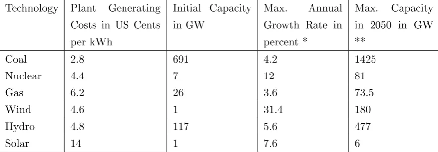
The technologies differ in three characteristics: (a) their marginal production costs, (b) their maximum annual capacity growth, and (c) the maximum possible capacity at the end of the time horizon. Table 1 shows the characteristics of the different tech-nologies. The data for maximal annual growth rate and maximum capacity in 2050 are based on data of the Energy Information Agency (2009). Additionally, we assume that with strong political support from the government growth rates can be 30 % higher, respectively a 50 % higher maximum capacity in 2050 than in the EIA (2009) scenario is possible.
To integrate those technological details in the general equilibrium model as described above, we coupled this bottom-up representation of the energy system with a top-down model of the macroeconomic environment in a complementarity framework, as it was developed by B¨ohringer and Rutherford (2008).
1
Technology Plant Generating Costs in US Cents per kWh
Initial Capacity in GW
Max. Annual Growth Rate in percent *
Max. Capacity in 2050 in GW **
Coal 2.8 691 4.2 1425
Nuclear 4.4 7 12 81
Gas 6.2 26 3.6 73.5
Wind 4.6 1 31.4 180
Hydro 4.8 117 5.6 477
[image:9.595.90.532.71.224.2]Solar 14 1 7.6 6
Table 1: Energy data. Based on data from the World Energy Outlook 2007 (IEA 2007) and International Energy Outlook 2009 (EIA 2009). *Growth rates from IEO (2009) plus 30 per cent. **Installed Capacity from IEO (2009) plus 50 per cent.
3.2 Modeling of Uncertainty
Investing in most long term projects such as power generation plants is beset with a substantial degree of uncertainty in the political framework. We incorporate these uncertainties through a stochastic decision problem. A single representative agent, which supplies labor and capital to the firms and is reimbursed with wage and capital income, maximizes expected utility,
max
Cs,t
E[U(Cs,t)], (6)
s.t. state-contingent market constraints such as:
As,t=Cs,t+Gs,t+Is,t+ X
j
Ij,s,tE . (7)
As,t is the available amount of the Armington good,Cs,t refers to consumption,Gs,t
is demand of the government, whereasIs,t denotes the investment in non-energy capital
and Ij,s,tE refers to the investment into energy technology j in year t and state of the worlds.2
Depending on expectations about the profitability, investors invest into the different technologies and build technology specific capital stocks. The technology specific capital stocks plus the capital stock used for the rest of the production in the economy are the state variables in our problem.
Once a investment is made in an specific technology this investment is irreversible. This provides a necessary condition for a proper modeling of the investment-under-uncertainty process. But not the whole amount invested is added to the capital stock. To depict a more realistic picture of investment decisions, which incorporate information-and transactions costs, we assume a distinction between net information-and gross investment as proposed by Uzawa (1969) in his quadratic adjustment cost formulation. To implement
2012 2020 2030 2040
2012
2030
[image:10.595.179.422.67.186.2]never
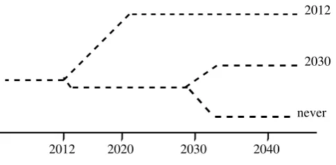
Figure 1: Stochastic event tree
the stochastic elements of the model, we use a set of new tools provided by Meeraus and Rutherford (2005).
The uncertainties that arise for the investor are depending on the actions of the government. Potential investors are uncertain if China’s government will, and if yes, when, introduces policy measures to reduce GHG emissions from power generation. We discuss the potential climate policy scenarios more in detail below.
Since the model has a finite time horizon but should be able to replicate the char-acteristics of an infinite horizon equilibrium we have to implement appropriate terminal conditions for the state variable and apply the strategy proposed by Lau, Pahlke, and Rutherford (2002).
3.3 Scenario Construction
Further necessary conditions to analyze the consequences of uncertainty are the oppor-tunity to time the investment and, obviously, uncertainty in future cash flows from the investment. Hence, recourse play a central role. The model is formulated as a decisions tree structure where we specify discrete probabilities of the events at every node in the decision tree.
Figure 1 shows the event tree. The future climate policy of China could take a con-tinuum of different forms. Along this concon-tinuum some architectures are more probable than others. Taking all different possible policy scenarios into account would obviously lead to a problem with very high dimensionality. We reduce the dimensionality of the model without a qualitative effect on our results and focus on three different potential policy scenarios. We could hence not capture the whole complexity of the problem and also the probability assumptions are chosen ad-hoc and do not depend on an elaborate analysis of the policy process. Since we are more interested in the fundamental mechanics of policy uncertainty we let these questions open for future research.
and reduce the emissions of greenhouse gases on the other, which let us conclude that the probability of this scenario might be around one third and assumePN ever = 0.35.
The two explicit climate policy scenarios are based on the two different policy archi-tectures examined in the Energy Modeling Forum (EMF) 22 modeling exercise (Clarke et al. (2009)). In the first climate policy scenario, called“2012”, roughly corresponding to the “full participation” scenario in Clarke et al. (2009), it is assumed that China joins a Post-Kyoto agreement and instantaneous participates in the efforts to stabilize emissions on the 450 ppm level to reach the two degree goal. In this case has China to reduce his emissions until 2020 by 22 per cent compared to the baseline. Most observers of China’s climate policy and of international climate negotiations judge the probabil-ity of an breakthrough in the negotiations as rather low. We attach a probabilprobabil-ity of
P2012 = 0.15 to this scenario.
The second policy architecture is softer in the transition to a global low carbon society. It respects the differentiated responsibilities in reducing emissions and enables China to delay the participation in a global climate agreement. This roughly corresponds to the policy architecture in the second EMF scenario, which stabilizes the atmospheric level of CO2 on 550 ppm. Under this scenario China has to start with its abatement
activities in 2030 and stabilize emissions ten percent below baseline in 2040. We call this scenario “2030” and deem it as rather probable. Hence, we attach a probability of
P2030 = 0.5 to this scenario.
3.4 Data
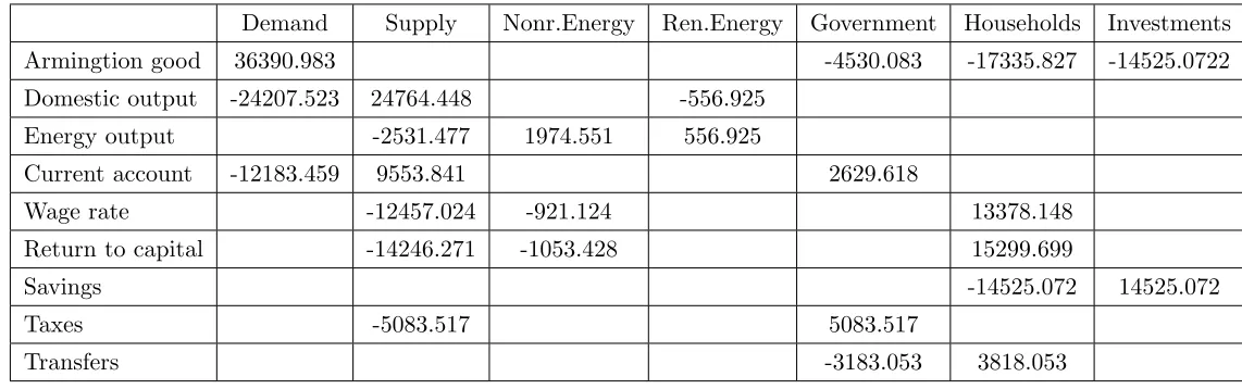
The micro-consistent social accounting matrix in Table 4 in the Appendix is based on data from the National Bureau of Statistics of China (2008). Information about growth capacities of the Chinese energy sector are taken from the International Economic Outlook 2009 of the Energy Information Agency. Data about cost structures and the current state of the Chinese energy sector are based on information from the World Energy Outlook 2007 from IEA (see Table 1).
To calibrate the dynamics of the model we use the parameters depicted in Table 6 in the Appendix. Assumption about the exogenous economic growth rate is based on calculations of the Energy Information Agency (2009).
4
Policy Simulations
4.1 The Consequences of Policy Uncertainty for the GHG Emission Path
Studying the CO2 emission path of the China’s power sector shows that without any
emission reduction policy GHG emissions would steadily increase and produce almost four gigatones of CO2 in 2040. This is almost four times the actual amount of emissions
to reduce their emissions. It shows the important role that China has if the problem of climate change should be solved.
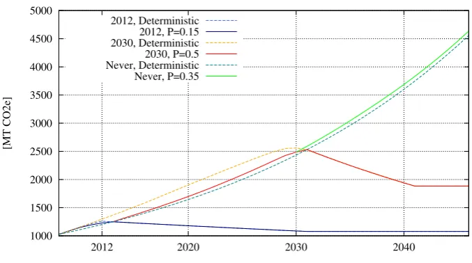
If China starts in 2030 reducing the emissions in the electricity sector, it could stabilize the emissions below two gigatones, which is still two times today’s amount. Starting already in 2012 would China allow to stabilize emissions approximately on the current level. But let us focus on the periods in advance of these key dates. Figure 2 depicts the emission path of China for all the discussed scenarios.
1000 1500 2000 2500 3000 3500 4000 4500 5000
[image:12.595.129.468.239.428.2]2012 2020 2030 2040
[MT CO2e]
Annual Emissions of GHG in the Electricity Sector
2012, Deterministic 2012, P=0.15 2030, Deterministic 2030, P=0.5 Never, Deterministic Never, P=0.35
Figure 2: GHG emission path in the power sector.
To examine the role of policy uncertainty we compare the outcome regarding emis-sions under perfect foresight, where the representative agent is perfectly informed on future climate policy decisions, with the outcome resulting from uncertainty of the way China’s government wants to deal with climate policy.
If we take a closer look on the emission path in the deterministic case, where the agent knows that emission reduction measures are implemented from “2030” onwards, we observe a substantial deviation to the emission path in the no-policy case. Relative to the outcome of the scenario“Never” emissions are significantly higher in periods before the policy implementation. Since the agent knows that the policy will be implemented, it is optimal to use as much as possible of the cheap energy, which coal provides as long its consumption is not regulated. During this pre-policy period, depending on the intertemporal elasticity of substitution, China is emitting between 12 and 14 % more than in the absence of any climate policy in later periods. Note that this difference due to the strong economic growth of china is tremendous.
30 35 40 45 50
P = 0 P = 1 P = 0.5
Gt CO
2
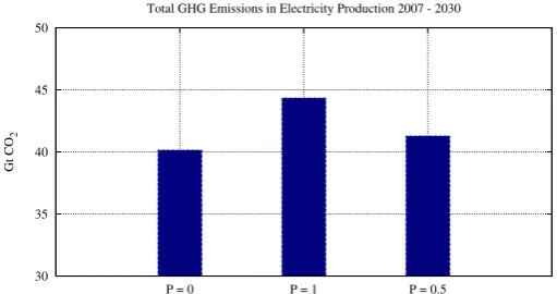
[image:13.595.170.426.95.230.2]Ex ante probability of climate policy implementation in 2030 Total GHG Emissions in Electricity Production 2007 - 2030
Figure 3: Sum of GHG emissions between 2007 and 2030.
periods. But let us now analyze the outcome under an uncertain implementation of climate policy. Studying the path in the stochastic case shows that after the policy implementation, emissions follow quickly the same path as in the deterministic cases. But in periods before the agent learns if the policy is implemented, GHG emissions are significantly lower than in the deterministic case. With only fifty percent change that in 2030 an abatement policy would be implemented and that the supply of cheap, coal-fired, energy might reduced, the pre-policy coal-fired energy becomes less valuable than in the deterministic case. The emissions are therefore due to the simple existence of uncertainty lower than under perfect information.
A further point supporting this argument is the observation that for higher intertem-poral elasticities of substitutions emissions are decreasing since it puts more weight on the expected consumption in the future in which maybe no reduction policy would take place. But the fact that the emissions in the stochastic cases are always higher than in “Never” indicates that the argument of exploiting cheap energy always dominates potential hedging investments in renewable energy technologies. If substantial hedging against the potential outcome of a stringent emission reduction policy would take place, emissions would be lower than in the deterministic case.
60% 80% 100%
E GAS HYDR NUCL SOLAR WIND 0% 20% 40% 60% 80% 100%
2012 2015 2018 2021 2024 2027
0% 20% 40% 60% 80% 100%
2030 2033 2036 2039 2042 2045 2048
80% 100% Scen: 2012 0% 20% 40% 60% 2007 2010 0% 20% 40% 60% 80% 100%
2012 2015 2018 2021 2024 2027
0% 20% 40% 60% 80% 100%
2030 2033 2036 2039 2042 2045 2048 0%
20% 40% 60%
2030 2033 2036 2039 2042 2045 2048
2012
Scen:
2030
Scen:
[image:14.595.123.482.86.347.2]never
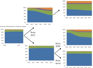
Figure 4: Energy mix along the stochastic event tree
4.1.1 Effects on the Technological Composition in the Power Sector
The amount of GHG emissions is obviously a function of the composition of the electricity sector. Figure 4 shows how the composition is evolving along the stochastic event tree. As the figures show, the composition does almost not react in advance of stochastic event nodes. Hence, the benefits from hedging against a potential regulation are smaller than the costs of this more expensive technologies. Changes in the composition starts only after the the introduction of binding emission reduction measures. In this case, the share of coal-fired power plants quickly decreases and hydro-electricity and to a smaller degree, nuclear and wind power increases their share. However, the transition in the energy sector takes only about ten to fifteen years, depending on the scenario. This might be a rather small period and obviously underestimates the long lead times for building, which are characteristic for most power plant projects. We let the consideration oft the “time to build” open for further research and concentrate us now on the evolving of composition of energy production.
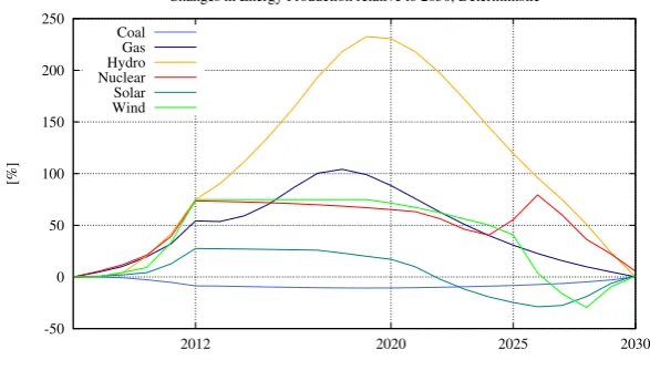
-50 0 50 100 150 200 250
2012 2020 2025 2030
[%]
Changes in Energy Production relative to 2030, Deterministic
[image:15.595.153.447.103.270.2]Coal Gas Hydro Nuclear Solar Wind
Figure 5: Changes in energy production per technology under uncertainty relative to the case where the implementation in 2030 is deterministic.
energy source, which reduces the emissions and more investments in renewables. But as already mentioned the increased investment in renewable energy technologies is not driven by an hedging rationale as we can see in Figure 6. Comparing the energy production under uncertainty with the energy production portfolio under the outcome with perfect knowledge that never a policy takes place shows that in this scenario invest-ments in renewables in pre-policy periods are lower and production of coal-fired power is higher. As this two comparisons show the incentive to maximize the potential utility from the cheapest energy source as long and intense as possible is clearly dominating any hedging rationale, which would lead to additional investment in clean energy sources.
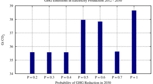
4.2 Sensitivity Analysis
To check the robustness of the results, a comprehensive sensitivity analysis of all crucial parameter values was carried out. Obviously, one of the central parameter which should affect the emission path in pre-policy periods is the probability distribution. We changed the subjective probability the representative agent had on the implementation of the scenario “2030”. Figure 7 shows the sum of emissions for different probabilities on scenario “2030”. Compared to the case where the probability of that event is equal to one, the sum of emissions in the electricity sector between 2012 and 2030 is always lower. However, in cases where the probability is between 0.5 and 0.6 emissions are significantly higher.
-80 -70 -60 -50 -40 -30 -20 -10 0 10
2012 2020 2025 2030
[%]
Changes in Energy Production relative to Scen. Never, Deterministic
[image:16.595.156.448.151.317.2]Coal Gas Hydro Nuclear Solar Wind
Figure 6: Changes in energy production per technology under uncertainty relative to the case where the agent knows that no climate policy will be implemented.
34 35 36 37 38 39
P = 0.2 P = 0.3 P = 0.4 P = 0.5 P = 0.6 P = 0.7 P = 1
Gt CO
2
Probability of GHG Reduction in 2030 GHG Emissions in Electricity Production 2012 - 2030
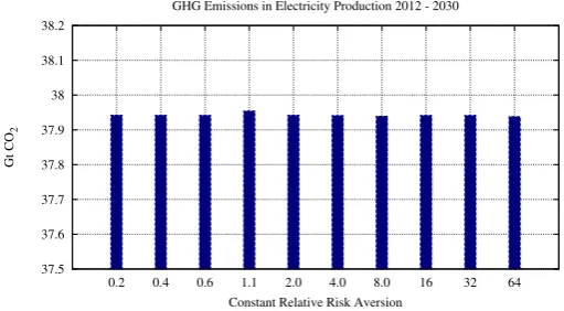
[image:16.595.170.427.514.655.2]37.5 37.6 37.7 37.8 37.9 38 38.1 38.2
0.2 0.4 0.6 1.1 2.0 4.0 8.0 16 32 64
Gt CO
2
[image:17.595.170.426.98.239.2]Constant Relative Risk Aversion GHG Emissions in Electricity Production 2012 - 2030
Figure 8: Total sum of GHG emissions for different values of constant relative risk aversion that China starts reducing GHG emissions in 2030.
regardless of the assumed risk aversion value.
5
Concluding Remarks
China is becoming the most important single energy market. The implementation of carbon abatement measures in China is therefore very important for the future success of any international climate agreement. But from the perspective of an investor, the signals from policy makers are not clear and he does not know if and when China will implement GHG emission reduction measures.
We study the role of this policy uncertainty for the investment in different energy technologies in China by the means of a stochastic general equilibrium model with an extended energy sector, which captures the most important characteristics of renewable and clean backstop technologies.
We see that under the assumption of perfect knowledge on the timing of the policy implementation, it becomes optimal for the representative agent to emit in pre-policy periods even more than in the absence of any policy intervention. The certain knowledge of the future scarcity of this source of energy makes it today more valuable and even causes an increase in investments in this sector in pre-policy periods.
Adding uncertainty about the if-and-when of the policy implementation dampens the expected present value of the cheap, but GHG emitting, coal-fired energy. Hence, emissions are in pre-policy periods lower than in the deterministic case of a certain policy implementation, but higher than in deterministic case where never such a policy takes place. The incentive to use cheap energy as long as possible does also dominate any hedging strategy.
benefits or the avoided damages in the environment for the utility of the representative agent, uncertainty causes obviously a decrease in welfare. But if we would incorporate environmental and climate damages in the utility or production function it could be possible to construct scenarios where such a policy uncertainty might be even welfare improving.
Since climate policy deals with long time horizons and is per se a complex issue compared to other policy fields, uncertainty for policy makers as well as for investors and consumers plays a crucial role. Further research in this evolving field is therefore necessary.
References
Arrow, K. J.(1968): “Optimal Capital Policy with Irreversible Investment,” inValue,
Capital and Growth, Papers in Honour of Sir John Hicks, ed. by J. Wolfe. Edinburgh University Press.
Black, F.,andM. Scholes(1973): “The pricing of options and corporate liabilities,”
The journal of political economy, 81(3), 637–654.
Blyth, W., R. Bradley, D. Bunn, C. Clarke, T. Wilson, and M. Yang(2007):
“Investment risks under uncertain climate change policy,”Energy policy, 35(11), 5766– 5773.
B¨ohringer, C.,andT. Rutherford(2008): “Combining bottom-up and top-down,”
Energy Economics, 30(2), 574–596.
BP (2009): “BP Statistical Review of World Energy 2009,” Discussion paper, British Petroleum.
Clarke, L., J. Edmonds, V. Krey, R. Richels, S. Rose, and M. Tavoni (2009):
“International climate policy architectures: Overview of the EMF 22 International Scenarios,” Energy Economics, 31, S64–S81.
Devarajan, S.,and D. Go(1998): “The simplest dynamic general-equilibrium model
of an open economy,” Journal of Policy Modeling, 20(6), 677–714.
Dixit, A.(1992): “Investment and Hysteresis,”Journal of Economic Perspectives, 6(1),
107–132.
Dixit, A., and R. Pindyck(1994): Investment under Uncertainty. Princeton
Univer-sity Press.
Energy Information Agency (2009): International Energy Outlook 2009. Energy
Information Agency.
Fuss, S., J. Szolgayova, M. Obersteiner, and M. Gusti (2008): “Investment
IEA(2007): World Energy Outlook 2007. OECD, Paris.
IEA (2010): “CO2 Emissions from Fuel Combustion - Highlights 2010,” Discussion paper, International Energy Agency.
Lau, M. I., A. Pahlke, and T. F. Rutherford (2002): “Approximating
Infinite-Horizon Models in a Complementarity Format: A Primer in Dynamic General Equi-librium Analysis,” Journal of Economic Dynamics & Control, 26, 577–609.
Laurikka, H.,andT. Koljonen(2006): “Emissions trading and investment decisions
in the power sector–a case study in Finland,”Energy Policy, 34(9), 1063–1074.
Meeraus, A., and T. Rutherford (2005): “Mixed complementarity formulations
of stochastic equilibrium models with recourse, Presentation at the GOR Workshop “Optimization under Uncertainty”, Bad Honnef, Germany (October 20?21, 2005).,” available at http://www.mpsge.org/StochasticMCP.ppt.
Merton, R.(1973): “Theory of rational option pricing,”The Bell Journal of Economics
and Management Science, pp. 141–183.
National Bureau of Statistics of China (2008): Chinese Statistical Yearbook
2008. Chinese State Statistical Publishing House, Beijing.
Pati˜no-Echeverri, D., P. Fischbeck, and E. Kriegler (2009): “Economic and
environmental costs of regulatory uncertainty for coal-fired power plants,” Environ-mental Science & Technology, 43(3), 578–584.
Peters, G., C. Weber, D. Guan, and K. Hubacek(2007): “China’s Growing CO2
Emissions - A Race between Increasing Consumption and Efficiency Gains,”Environ. Sci. Technol, 41(17), 5939–5944.
Pindyck, R. (1991): “Irreversibility, Uncertainty, and Investment,” Journal of
Eco-nomic Literature, 29(3), 1110–1148.
Rutherford, T. (1995): “Extension of GAMS for complementarity problems arising
in applied economic analysis,” Journal of Economic Dynamics and Control, 19(8), 1299–1324.
Uzawa, H. (1969): “Time preference and the Penrose effect in a two-class model of
economic growth,” The Journal of Political Economy, 77(4), 628–652.
Zhou, W., B. Zhu, S. Fuss, J. Szolgayov´a, M. Obersteiner,andW. Fei(2010):
Appendix
A
Calibration
A.1 Parameters
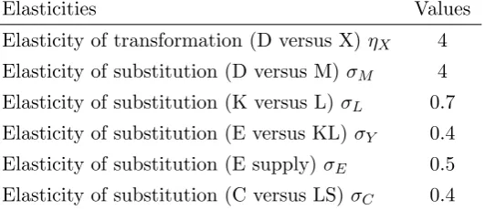
Elasticities Values
Elasticity of transformation (D versus X)ηX 4
Elasticity of substitution (D versus M)σM 4
Elasticity of substitution (K versus L)σL 0.7
Elasticity of substitution (E versus KL)σY 0.4
Elasticity of substitution (E supply)σE 0.5
[image:20.595.168.434.166.281.2]Elasticity of substitution (C versus LS)σC 0.4
Table 2: Elasticities of transformation and substitution, respectively.
Parameter Values
Benchmark Interest Rater0 0.05 Depreciation Rateδ 0.07
Growth Rateσ 0.04
Adjustment Costs Intensityφ 0.3 Intertemporal Elasticity of SubstitutionσT 0.5
Constant Relative Risk AversionσR 1.1
[image:20.595.166.434.328.446.2]B
Equations in the Model
B.1 Zero Profit Conditions
Zero profit in the macro good production:
ΠYs,t(θZpXt,s
(1+ηx)
+ (1−θZ)pDt,s(1+ηx))1+1ηx −
θYKL1−σY
t,s + (1−θY)pEt,s
1−σY 1 1−σY
= 0,
(8) where KLt,s=
θKw1−σK
t,s + (1−θK)rk1− σK t,s
1 1 −σK.
Zero profit in consumption good:
ΠAs,t=pAt,s−
θMpMt,s
1−σM
+ (1−θM)pDt,s
1−σM 1 1−σM
= 0. (9)
Zero profit in coal-fired power generation:
ΠCs,t=pEt,s−θECw1−σE
t,s + (1−θEj )rkEC,t,s
1−σK 1
1−σE) +ψ
CpCO2s,t +p QI
C,t,s= 0, (10)
where ψj denotes the greenhouse gas emission coefficient per technology j.
Zero profit in backstop technologies:
ΠBs,t=pEs,t+X
sw
νl,t+1,sw(1 +γl)−θBl rkj,t,sE +θ Q l p
Q l,t,s+θ
Q
l νl,t,s+ψlpCO2 = 0. (11)
Zero profit in the capital markets:
pKt,s = X
sow
pKtt+1,sow(1−δ) +rktt,s+pKAtt,s (12)
pKEt,s = X
sow
pKEtt+1,sow(1−δ) +rkEtt,s+pKAtt,s (13)
(14)
Zero profit for investments:
ΠIs,t = X
sw
pKt+1,sw−pAt,s+ 2(pkt,sA0.5+pAt,s0.5) = 0 (15)
ΠIEj,s,t = X
sw
pKEj,t+1,sw−pAt,s+ 2(pkt,sA0.5+pAt,s0.5) = 0 (16)
Zero profit for the final consumption good including consumption - leisure choice:
ΠLSs,t =X
sw
pCt,sw−θCpAt,s1−σ+ (1−θc)w1−σ t,s
11 −σ
= 0 (17)
B.2 Market Clearing Conditions
Market clearing for the consumption good:
At,s=Gt,s+Ct,s+It,s+ X
j
Demand Supply Nonr.Energy Ren.Energy Government Households Investments Armingtion good 36390.983 -4530.083 -17335.827 -14525.0722 Domestic output -24207.523 24764.448 -556.925
Energy output -2531.477 1974.551 556.925
Current account -12183.459 9553.841 2629.618
Wage rate -12457.024 -921.124 13378.148
Return to capital -14246.271 -1053.428 15299.699
Savings -14525.072 14525.072
Taxes -5083.517 5083.517
[image:22.842.133.704.182.361.2]Transfers -3183.053 3818.053
Table 4: Micro consistent Social Accounting Matrix. Depends on data from the Statistical Yearbook of China 2008 of the Chinese National Bureau for Statistics and from the International Energy Outlook of EIA 2009. All values are 100 Millions of US Dollars 2008
Us Utility from states
Ct,s Consumption in timetand state s
Yt,s Goods production in timet and state s
At,s Armington good in timet and state s
Mt,s Imports in timetand state s
Xt,s Exports in timet and states
Ej,t,s Electricity from technology j in timetand state s
Bj,t,s Backstop technologyj in time tand state s
Kt,s, Conventional capital stock in timetand state s
KEj,t,s Capital stock for energy j in timetand state s
It,s Investment in conventional capital stock in timetand state s
[image:23.595.116.486.103.312.2]IEj,t,s Investment in energy capital stock of tech. j in time tand state s
Table 5: List of the activity levels
pUs Price of utility from state s
pCt,s Price of consumption good in time tand state s
pGCt,s Shadow price of gross consumption in timet and state s pDt,s Domestic Price of output in time tand state s
pA
t,s Price of Armington good in timet and state s
pMt,s Import price index in timet and states pXt,s Export price in timet and state s pEj,t,s Price of Energy in timet and state s pLt,s Wage rate index in time tand state s rK
t,s Rental rate index in time tand state s
rj,t,sKE Rental rate for energy capitalj in time tand state s pKt,s Purchase price of capital in time tand state s
pKEj,t,s Purchase price of energy capital j in timet and states pAKt,s Premium for Capital adjustment costs in time tand state s pF
t,s Foreign exchange rate
pCOt,s 2 Carbon price in timet and state s
νj,t,s Shadow price of growth limit of tech. j in timetand state s
pQj,t,s Shadow price of quota limit of tech. j in time tand state s
Market clearing in the goods market:
∂ΠY s,t
∂pD s,t
= ∂Π
A s,t
∂pD s,t
(19)
Market clearing for the import good:
Mt,s=
∂ΠA s,t
∂pM s,t
(20)
Market clearing for the export good:
∂ΠY s,t
∂pYs,t =Xt,s (21)
Market clearing in the energy market:
∂ΠY s,t
∂pE s,t
=X
j
Ej,t,s+ X
l
Bl,t,s (22)
Market clearing capital markets
Kt,s =
∂ΠYs,t
∂rks,t
(23)
KEj,t,s =
∂ΠCs,t
∂rkC,s,tE +Bj,t,s (24)
Capital accumulation
Kt−1,s(1−δ) +It−1,s = Kt,s (25)
KEj,t−1,s(1−δ) +IEj.t−1,s = KEj,t,s (26)
Market clearing carbon market
CO2s,t = X
j
ψj(Ej,t,s+Bj,t,s), (27)
whereas CO2s,t describes the cap on CO2 emissions in statesat timet.
Market clearing labor market
Ls,t=
∂ΠYs,t
∂ws,t
(28)
Income household
HH=X
s X
t
wt,s+pK0,sK0,s+pj,KE0,sKEj,0,s+pCO2t,s CO2s,t
(29)
Terminal capital constraints
Itl,s
Itl−1,s
= Atl,s
Atl−1,s
∀t > T (30)
IEj,tl,s
IEj,tl−1,s
= Atl,s
Atl−1,s
∀t > T, (31)
(32)