The effects of real exchange rate misalignment and real exchange volatility on exports

(1)

The effects of real exchange rate

misalignment and real exchange volatility

on exports

Diallo, Ibrahima Amadou

Clermont University, University of Auvergne, Centre d’Etudes et de

Recherches sur le Développement International, CERDI

30 April 2011

Online at

https://mpra.ub.uni-muenchen.de/32387/

(2)

The Effects of Real Exchange Rate

Misalignment and Real Exchange

Volatility on Exports

Diallo Ibrahima Amadou

1

April, 2011

Abstract

This paper uses panel data cointegration techniques to study the impacts of real exchange rate misalignment and real exchange rate volatility on total exports for a panel of 42 developing countries from 1975 to 2004. The results show that both real exchange rate misalignment and real exchange rate volatility affect negatively exports. The results also illustrate that real exchange rate volatility is more harmful to exports than misalignment. These outcomes are corroborated by estimations on subsamples of Low-Income and Middle-Income countries.

Keywords: real effective exchange rate; misalignment; volatility; exports; pooled mean group estimator

JEL Classification: F13, F31, F41

1

(3)

Introduction

Theoretically, real effective exchange rate (REER) misalignment has a negative effect on

economic performance. In fact, it reduces the export of tradable goods and the profitability of

production. REER misalignment deteriorates domestic investment and foreign direct investment,

consequently growth, by increasing uncertainty. REER misalignment leads also to a reduction in

economic efficiency and a misallocation of resources (Edwards (1988), Cottani, et al. (1990) and

Ghura and Grennes (1993)). Studies have also shown that undervaluation can improve growth.

Levy-Yeyati and Sturzenegger (2007) state that undervaluation increases output and productivity through an expansion of savings and capital accumulation. Rodrik (2009) illustrates that undervaluation rises the profitability of the tradables sector, and leads to an extension of the

share of tradables in domestic value added. Larger profitability encourages investment in the

tradables sector and helps economic growth. Korinek and Serven (2010) illustrates that real exchange rate undervaluation can increase growth through learning-by-doing externalities in the

tradables sector.

Real effective exchange rate (REER) volatility has also a negative impact on economic

performance. In fact, higher REER instability raises uncertainty on the profitability of producing

tradable goods and of long-run investments. Higher REER volatility sends confusing signals to

economic agents (Grobar (1993), Cushman (1993) and Gagnon (1993)). Some authors, like

Aghion et al. (2009), have argued that the impact of exchange rate volatility on economic performance is function of the level of financial development. Others states that the effect of

exchange rate variability on economic performance depends on the complementarity between

(4)

Many studies have investigated the empirical link between exchange rate misalignment,

REER volatility and economic performance in general and between REER misalignment and

exports in particular. Cottani et al. (1990), Razin and Collins (1997) and Aghion et al. (2009) show that there exists a negative correlation between REER volatility or REER misalignment

and economic performance. For the link REER misalignment-export, using a panel data of 53

countries Nabli and Véganzonès-Varoudakis (2002) found a negative relationship. The same results were found by Jongwanich (2009) for a sample of Asian developing countries. Sekkat and Varoudakis (2000) found that REER volatility does not have a systematic negative impact on manufactured export while REER misalignment exerts a significant negative influence on export

for a panel of Sub-Saharan African countries. Jian (2007) also found that exchange rate

misalignment has a negative influence on China’s export.

This paper fits in these researches of the links between the REER misalignment, REER

volatility and economic performance. It specifically analyzes the relationship between exchange

rate misalignment, REER volatility and total exports. It distinguishes itself by using panel data

cointegration techniques and a measurement of REER volatility which have not been used in

previous works. The sample studied contains 42 developing countries from 1975 to 2004. We

use panel data cointegration techniques because our time span is too large: 30 years. This raises

the question of the existence of potential unit root in the variables studied and leads to the issue

of cointegration. The application of panel data cointegration techniques has several advantages.

Initially, annual data enable us not to lose information contrary to the method of averages over

subperiods. Then, the addition of the cross sectional dimension makes that statistical tests are

normally distributed, more powerful and do not depend on the number of regressors in the

(5)

Pesaran et al. (1999) Pooled Mean Group Estimation of Dynamic Heterogeneous Panels

estimator. The microeconomic panel data methods: random effects, fixed effects, and GMM

oblige the parameters (coefficients and error variances) to be identical across groups, but the

intercept can vary between groups. GMM estimation of dynamic panel models could lead to

inconsistent and misleading long-term coefficients when the period is long. Pesaran et al. (1999)

suggest a transitional estimator that permits the short-term parameters to differ between groups

while imposing equality of the long-run coefficients.

The paper is organized as follow: section 1 presents the econometrics estimations

methods, section 2 analyze the data, section 3 shows how the variables of interests are measured,

section 4 and 5 deal with the panel data tests and main estimations results respectively, section 6

(6)

1. Econometrics models and estimations methods

To estimate the effect of exchange rate misalignment, REER volatility on total exports,

the method of Pooled Mean Group Estimation of Dynamic Heterogeneous Panels of Pesaran et al. (1999) is applied. In this model, the long-run variation of export and other regressors are supposed to be identical for countries but short-run movements are expected to be specific to

each country. The estimated model is an



ARDL





p q, ,...,₁ _qk



representation of the form:

(1)

, ,

1 0 ij

p q

y_it _{ij i t j}y X_{i t j} _i _it

j j

   

       

 

Where i1, 2,...,Nis the number of groups; t1, 2,...,Tis the number of periods; _Xitis the k1vector of regressors;

ij

 are the k1 coefficient vectors; ij

 are scalars and _iis the

fixed effects.

Equation (1) can be rewritten as error correction model of the form:





1 * 1 '* ₍₂₎

, 1 , 1 _,

1 0

i

p q

y_it _i y_{i t} X_it _ij y_{i t} _ij X_{i t j} _i _it

j j                    _     Where 1 1 p i ij j     _  _ 

 ; 0 / 1

q

i _j ij _k ik

    _  _

  ;

*

1, 2,..., 1 1

p

j p ij _{m j} im

      

 

and * 1, 2,..., 1

1 q j q ij im m j          .

The parameter _iis the error correction term. This parameter is supposed to be significantly negative since it is assumed that the variables return to a long-term equilibrium. The

long-run relationships between the variables are in the vector '

i

 . To estimate equation (2)

(7)

coefficients to be equal through the groups but forces short-term coefficients and error variances

to be different through the groups. Pesaran et al. (1999) use the maximum likelihood method to estimate the parameters in equation (2) given that this equation is nonlinear. The log-likelihood

function is given by:

 

₂ 1 1



 





 



( , , ) ln 2 (3)

2

2 1 2 1

N N

T

l _i y_i _{i i} H_i y_i _{i i}

T _i _i

i                          

Where i1,...,N;

 

, 1

y X i i t i i

   _   ; H_i I_T W W W W_i



_i _i



_i, I

Tis an identity matrix of

order T and



,..., , , ,...,



, 1 , 1 , 1 , 1

W_i y y X_i X X i t i t p i t i t q

  _  _{ }   _  _{ } .

The estimated long-run relationship between REER misalignment, REER volatility, the

control variables and exports is:

0 1 2 3 4

5 6 7

( ) ( ) ( )

( ) ( ) ( ) (4)

it it it it it

it it it it

Log EXPGDP MISAL RERVOL Log MVADGDP Log GDPTP Log TOT Log RGDP Log INVGDP

    

   

     

  

Where _i are the long-term parameters, Log EXPGDP( it) is Log Exports to GDP,

it

MISAL is REER misalignment, RERVOLit is REER volatility, Log MVADGDP( it) Log Manufactured value added to GDP, Log GDPTP( it) Log GDP of trade partners, Log TOT( it) Log Terms of trade, Log RGDP( it) Log Real GDP and Log INVGDP( it) Log Investment to GDP. Table 1 gives the definition, expected signs and sources of all variables of the study and Table 2

shows the summary statistics on the variables. If we assume that all variables in equation (4) are

(8)

1 0 1 2 3

4 5 6 7

( ) [ ( ) ( )

( ) ( ) ( ) ( )]

+

it i it it it it

it it it it

Log EXPGDP Log EXPGDP MISAL RERVOL Log MVADGDP Log GDPTP Log TOT Log RGDP Log INVGDP

    

   



     

   

1 2 3 4

5 6 7

( ) ( )

+ ( )+ ( )+ ( ) (5)

i it i it i it i it

i it i it i it it

MISAL RERVOL Log MVADGDP Log GDPTP Log TOT Log RGDP Log INVGDP

   

   

      

   

The parameter i is the error-correcting speed of adjustment term. As mentioned above,

we expect this parameter to be significantly negative implying that variables return to a long-run

equilibrium.

2. Data and Variables

To study the eﬀect of REER misalignment and REER volatility on exports, we utilize

annually data from 1975 to 2004 of 42 developing countries. The data are from World

Development Indicators (WDI) 2006, International Financial Statistics (IFS), April, 2006 and

Centre D’études Et De Recherches Sur Le Développement International (CERDI) 2006. Table 3

gives the list of all countries used in the study.

The REER is calculated according to the following formula:

10 (6) / / ₁ j CPIi

RER _{NBER j i}

i j _j _{CPI j}

            Where: / NBER

j i: is the nominal bilateral exchange rate of trade partner j relative to countryi

CPIi: represents the consumer price index of country i (IFS line 64). When the country CPIis

(9)

CPI j: corresponds to the consumer price index of trade partner j (IFS line 64). When the country CPIis missing, the growth rate of the GDP deﬂator is used to feel the data;

j

 : stands for trade partner j weight (mean 1999-2003, PCTAS-SITC-Rev.3). Only the ﬁrst ten

partners are taking (CERDI method). These first ten partners constitute approximately 70% of

trade weights. The weights used to generate the REER are (Exports + Imports) / 2 excluding oil countries. Weights are computed at the end of the period of study in order to focus on the

competitiveness of the most recent years.

An increase of the REER indicates an appreciation and, hence a potential loss of

competitiveness.

3. Measurement of variables of interest

In this section, we will present how the variables of interest are calculated.

3.1.Measurement of REER Misalignment

Before calculating the REER misalignment, we first compute the equilibrium real

exchange rate (EREER). The economic literature on exchange rate states that REER is affected

by its determinants called “fundamentals” (Williamson (1994), Edwards (1998)). We use the PMG estimator to estimate the relationship between REER and its fundamentals. The long-run

estimated equation is:

0 1 2 3

( _it) ( _it) ( _it) ( _it) _it (7)

(10)

Where Log REER( it) is the logarithm of real effective exchange rate, Log TOT( it)the log of terms of trade, Log GDPCAP( it) the log of real GDP per capita and Log OPEN( it)is the log of export and import over GDP.

We expect that a rise in terms of trade ameliorates trade balance, the income effect

dominating the substitution effect, hence ₁ is expected to be positive. GDP per capita captures

the Balassa-Samuelson effect which states that productivity increases faster in tradable than in non-tradable sectors. This phenomenon augments wages in the tradable sector, consequently

wages in the non-tradable sector. This implies an increase in domestic inflation and an

appreciation of the REER. Hence we expect ₂ to be positive. Restricted trade has a downward

effect on the relative price of tradable to non-tradable goods, leading therefore to an appreciation

of the REER. Thus ₃ is supposed to be negative.

If we assume that all variables in equation (7) are I(1) and cointegrated then _it is I(0).

The error correction representation of equation (7) is given by:



1 0 1 2 3



1 2 3

( ) ( ) ( ) ( ) ( )

+ ( ) ( ) ( ) (8)

it i it it it it

i it i it i it it

Log REER Log REER Log TOT Log GDPCAP Log OPEN

Log TOT Log GDPCAP Log OPEN

    

   



     

     

The parameter _i is the error-correcting speed of adjustment term. As mentioned above,

we expect this parameter to be significantly negative implying that variables return to a long-run

equilibrium. Of particular importance are the parameters i which capture the long-term

relationship between REER and the fundamentals. The results of the estimation of equation (8)

(11)

Table 4 shows that all parameters have the expected signs and are statistically significant.

In particular the Adjustment coefficient is negative. This relationship between REER and the

fundamentals is also cointegrated. For example the Pedroni (1999) panel data cointegration Panel-PP statistic and Group PP-statistic are respectively 0.0121 and 0.0178. This result and the

negative sign of the Adjustment coefficient mean that the long-run value of REER stays around

its equilibrium value. After estimating equation (8), we multiply the parameters _i by the

corresponding three year moving average of the corresponding fundamental. This result gives us

the equilibrium REER (EREER). Then REER misalignment is then computed according to the

following formula:

( )

1 (9)

( ) it it it Log REER Misal Log EREER  

In equation (9), a positive value of Misalit represents an overvaluation.

3.2.Measurement of REER Volatility

We compute real exchange rate volatility using ARCH family methods. Specifically we

apply the asymmetric EGARCH (1, 1). The asymmetry implies that positive values of residuals

have a different effect than negative ones. This is formulated as below:

1 0

1

2 2 1

t 0 1 ₂ 1 1 1 ₂

1 1

( ) ( )

( ) ( ) (10)

t t t

t t

t

t t

Log REER Log REER

Log Log                         

Where t are distributed as

2 t

(0, )

N  , 2

t

 the variance of the regression model’s

disturbances, _i the ARCH parameters, ₁ the GARCH parameter, ₁ the asymmetric EGARCH

(12)

produce higher variances in the near future. We measure the exchange rate volatility as the

square root of the variance of the regression model’s disturbances.

4. Panel data tests

In this section, we will successively present the panel unit root tests and the cointegration

tests.

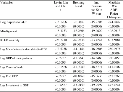
4.1.Panel Unit Root Tests

Table 5 gives the results of the unit root tests for all variables expressed in level. In all

tests, the null hypothesis is that the series contains a unit root, and the alternative is that the series

is stationary. The Levin, Lin and Chu and the Breitung tests make the simplifying assumption that the panels are homogenous while the other tests assume that the panels are heterogeneous.

Excluding Log Investment to GDP and REER volatility which are stationary2, the tests show that

all the other variables may contain unit root. Moreover Table 6 illustrates that these other

variables are potentially I(1). This last result leads us to the issue of cointegration among these variables.

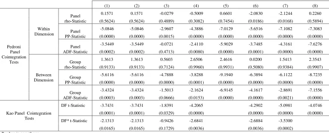
4.2.Panel Cointegration Tests

Table 7 shows the panel data cointegration tests for the equations used in the main

estimation results3. Among the panel cointegration tests, we utilize the Pedroni (1999) and Kao

2

The Misalignment variable can also be considered as stationary because two tests out of four show that it is stationary.

3

(13)

(1999) panel cointegration tests. In the Pedroni (1999) tests, the first three tests present the within dimension while the others give the between dimension. For the Kao (1999) tests, only the Dickey-Fuller type tests are shown. In all these tests, the Null Hypothesis is that there is No

cointegration. Overall, the results illustrates that there exist a cointegration relationship for all

equations.

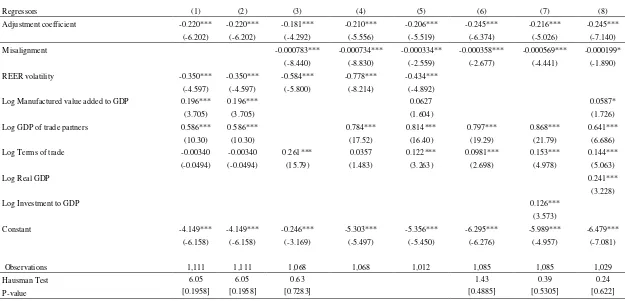
5. Estimation Results

Table 8 presents the main estimation of the long-term coefficients that interest us. We

know that the PMG estimator constrains the long-run elasticities to be equal across all panels.

This PMG estimator is efficient and consistent while the Mean Group (MG) estimator, which

assumes heterogeneity in both short-run and long-run coefficients, is consistent when the

restrictions are true. If the true model is heterogeneous, the PMG estimator is inconsistent while

the MG estimator is consistent. We run a Hausman test to test for the difference between these two models in our sample of study. The P-values for the Hausman test in Table 8 show that we do not reject the Null hypothesis that the efficient estimator, the PMG estimator, is the desired

one. The speed of adjustment parameter is negative and highly significant in all regressions and

is approximately stable in magnitude. As mentioned above, this result suggests that the variables

return to a long-run equilibrium.

All eight equations in Table 8 illustrate that REER misalignment and REER volatility are

statistically signiﬁcant and have the expected signs. We notice that the magnitude of REER

misalignment is too low compared to that of REER volatility. This suggests that REER volatility

(14)

volatility is very high. Referring to regression 4, an increase in REER volatility by one standard

deviation reduces the ratio of exports to GDP by an amount approximately equivalent to 24%.

These results corroborate those found by several studies like Ghura and Grennes (1993) and

Grobar (1993). The absolute value of the REER volatility coeﬃcient diminishes by half when we introduce the logarithm of GDP of trade partners in regressions 1, 2 and 5, suggesting that the

eﬀect of volatility on exports may pass through the GDP of trade partners.

The results also highlight that exports are positively influenced by manufactured value added

to GDP, GDP of trade partners, Real GDP and Investment to GDP. The Terms of trade, when they

are significant, are also positively related to exports. The positive value of the coefficient of GDP of

trade partners means that when the trade partners experience high growth, this results in a pulling

effect on the exports of the home country. The positive effect of Real GDP and Investment to GDP

means that exports increase when the productive capacity of a country rises.

6. Robustness Analysis

Table 9 and 10 give the estimations of the effects of REER misalignment and REER

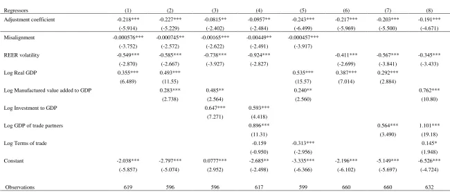
volatility on exports for the low income and middle income developing countries respectively.

The results in the two table show that both REER misalignment and REER volatility affect

negatively exports. This confirms the findings of our main estimations results. Also as in the

main estimations, we observe that REER volatility has is more harmful to exports than

(15)

Conclusion

We studied the effects of REER misalignment and REER volatility on exports for 42

developing countries from 1975 to 2004. Using new developments on panel data cointegration

techniques, we found that both REER misalignment and REER volatility have a strong negative

impact of exports. But the effect of REER misalignment is smaller than that of REER volatility.

The impact of REER volatility is very high: an increase in REER volatility by one standard

deviation reduces the ratio of exports to GDP by an amount approximately equivalent to 24%.

Although the results found were informative, some caveats remain. First, we did not

analyze the effect of REER misalignment and REER volatility on manufactured exports and for

developed countries. Second, the fact that REER misalignment is a generated regressor could

cause some bias in the estimation results, especially in the standards errors of the regressions.

From policy perspectives, the results show that macroeconomic instability, in particular

exchange rate volatility could have negative impacts on exports and that efforts made to reduce

(16)

References

Aghion, P., Bacchetta, P., Ranciere, R. and Rogoff, K.: 2009, Exchange Rate Volatility and Productivity Growth: The Role of Financial Development, Journal of Monetary Economics 56 (4), 494–513.

Cottani, J. A., Cavallo, D. F. and Khan, M. S.: 1990, Real Exchange Rate Behavior and Economic Performance in LDCs. Economic Development and Cultural Change 39. Cushman, D. O.: 1993, The Effects of Real Exchange Rate Risk on International Trade. Journal

of International Economics 15.

Edwards, S.: 1988, Exchange Rate Misalignment in Developing Countries, Baltimore: The Johns Hopkins University Press.

Edwards, S.: 1998, Capital Flows, Real Exchange Rates, and Capital Controls: Some Latin American Experiences, NBER Working Papers 6800.

Eichengreen, B.: 2008, The Real Exchange Rate and Economic Growth, Working Paper No. 4.

Commission on Growth and Development, World Bank, Washington, Dc.

Gagnon, J. E.: 1993, Exchange Rate Variability and the Level of International Trade. Journal of International Economics 34(3-4).

Ghura, D. and Grennes, T. J.: 1993, The Real Exchange Rate and Macroeconomic

Performances in Sub-Saharan Africa, Journal of Development Economics 42.

Ghura, D. and Grennes, T. J.: 1993, The Real Exchange Rate and Macroeconomic

Performances in Sub-Saharan Africa. Journal of Development Economics 42.

Grobar, L. M.: 1993, The Effect of Real Exchange Rate Uncertainty on LDC Manufactured Exports. Journal of Development Economics 14.

Grobar, L. M.: 1993, The Effect of Real Exchange Rate Uncertainty on LDC Manufactured Exports, Journal of Development Economics 14.

Jian, L.: 2007, Empirical study on the influence of RMB exchange rate misalignment on China’s export-Based on the perspective of dualistic economic structure, Front. Econ. China 2(2), 224–236.

Jongwanich, J.: 2009, Equilibrium Real Exchange Rate, Misalignment, and Export Performance in Developing Asia, ADB Economics Working Paper Series No. 151.

Kao, C.: 1999, Spurious Regression and Residual-Based Tests for Cointegration in Panel Data,

(17)

Korinek, A. and Serven, L.: 2010, Undervaluation through Foreign Reserve Accumulation: Static Losses, Dynamic Growth, Policy Research Working Paper 5250, World Bank, Washington, DC.

Levy-Yeyati, E. and Sturzenegger, F.: 2007, Fear of Appreciation, Policy Research Working Paper 4387, World Bank, Washington, DC.

Nabli, M. K. and Véganzonès-Varoudakis, M-A.: 2002, Exchange Rate Regime and

Competitiveness of Manufactured Exports: The Case of MENA Countries, Working Paper, The World Bank.

Pedroni, P.: 1999, Critical Values for Cointegration Tests in Heterogeneous Panels with Multiple Regressors, Oxford Bulletin of Economics and Statistics 61, 653–70.

Pesaran, M. H., Shin, Y. and Smith, R. P.: 1999, Pooled mean group estimation of dynamic heterogeneous panels, Journal of the American Statistical Association 94, 621-634.

Razin, O. and Collins, S. M. A.: 1997, Real Exchange Rate Misalignments and Growth, NBER

Working Paper no. 6174.

Rodrik, D.: 2009, The Real Exchange Rate and Economic Growth, In Brookings Papers on Economic Activity, Fall 2008, ed. D. W. Elmendorf, N. G. Mankiw, and L. H. Summers, 365–412. Washington, DC: Brookings Institution.

Sekkat, K. and Varoudakis, A.: 2000, Exchange rate management and manufactured exports in

Sub-Saharan Africa, Journal of Development Economics 61 (2000), 237–253.

(18)

[image:18.612.74.543.111.367.2]

Table 1: Definitions and methods of calculation of the variables

Variables Definitions

Expected

Sign Sources of data

Log Exports to GDP Total Exports divided by GDP

Log Manufactured value added to GDP

Logarithm of Manufactured value added over GDP

Positive World Bank, World Development Indicators, 2004

Log GDP of trade partners

Logarithm of the GDP of trade partners. The trade partners are the same as those used to calculate the REER

Positive Author

calculations

Log Terms of trade Logarithm of the terms of trade Positive or Negative

World Bank, World Development Indicators, 2004

Log Real GDP Logarithm of the real GDP Positive

Log Investment to

GDP Logarithm of the total Investment to GDP Positive

Table 2: Summary statistics on variables

Variables Obs. Mean Std. Dev. Min Max

Log Exports to GDP 1259 -1.4201 0.6245 -3.5422 0.2184

Misalignment 1136 23.2513 896.0622 -8108.7380 27431.8100

REER volatility 1241 0.1531 0.3056 0.0003 7.1438

Log Manufactured value added to GDP 1185 -1.9430 0.4992 -3.6892 -0.8988

Log GDP of trade partners 1260 30.3331 1.1001 26.5335 32.3573

Log Terms of trade 1249 0.0517 0.2627 -0.9333 1.8050

Log Real GDP 1260 22.9255 1.9825 18.5565 28.1704

[image:18.612.79.537.432.570.2]

(19)

[image:19.612.73.530.116.463.2]

Table 3: List of 42 countries

No. World Bank Code Countries No. World Bank Code Countries

1 ARG Argentina 22 HND Honduras

2 BDI Burundi 23 HUN Hungary

3 BEN Benin 24 IDN Indonesia

4 BFA Burkina Faso 25 IND India

5 BGD Bangladesh 26 KEN Kenya

6 BOL Bolivia 27 LKA Sri Lanka

7 CHL Chile 28 LSO Lesotho

8 CHN China 29 MAR Morocco

9 CIV Cote d'Ivoire 30 MEX Mexico

10 CMR Cameroon 31 MLI Mali

11 COG Congo, Rep. 32 MRT Mauritania

12 COL Colombia 33 MWI Malawi

13 CRI Costa Rica 34 MYS Malaysia

14 DOM

Dominican

Republic 35 NIC Nicaragua

15 DZA Algeria 36 PER Peru

16 ECU Ecuador 37 PHL Philippines

17 GAB Gabon 38 PRY Paraguay

18 GHA Ghana 39 SEN Senegal

19 GMB Gambia, The 40 SWZ Swaziland

20 GNB Guinea-Bissau 41 TGO Togo

(20)

[image:20.612.199.413.129.317.2]

Table 4: Estimation of Equilibrium Real Exchange Rate (EREER)

Dependent Variable: Log(REER)

Regressors Adjustment coefficient -0.136***

(-7.470)

Log Terms of trade 0.343*** (8.811) Log Real GDP per Capita 0.156* (1.911) Log Openness -0.268***

(-4.432) Constant 0.487***

(7.151)

Observations 1,085 z-statistics in parentheses

(21)

[image:21.612.90.526.115.410.2]

Table 5: Panel unit root tests (Level of variables)

Variables Levin, Lin

and Chu t

Breitung t-stat

Im, Pesaran and Shin

W-stat

Maddala Wu ADF-Fisher

Chi-square

Log Exports to GDP 0.4990 -12.8756 -1.1752 70.0695

(0.6911) (0.0000) (0.1200) (0.8618)

Misalignment -1.1166 -4.2965 -14.4034 16.3843

(0.1321) (0.0000) (0.0000) (0.1743)

REER volatility -19.5993 -12.8756 -15.7458 277.0994

(0.0000) (0.0000) (0.0000) (0.0000)

Log Manufactured value added to GDP -1.0035 1.5786 -1.0080 103.0233

(0.1578) (0.9428) (0.1567) (0.0014)

Log GDP of trade partners 1.3394 3.7455 3.4090 53.9241

(0.9098) (0.9999) (0.9997) (0.9956)

Log Terms of trade -1.1245 -0.0145 -2.5253 111.3942

(0.1304) (0.4942) (0.0058) (0.0032)

Log Real GDP -1.0386 -0.2293 1.9469 87.8968

(0.1495) (0.4093) (0.9742) (0.3080)

Log Investment to GDP -5.4324 -3.9206 -5.7130 178.3153

(0.0000) (0.0000) (0.0000) (0.0000)

(22)

[image:22.612.100.516.112.423.2]

Table 6: Panel unit root tests (First Difference of variables)

Variables Levin, Lin

and Chu t

Breitung t-stat

Im, Pesaran and Shin

W-stat

Maddala Wu ADF-Fisher Chi-square

Log Exports to GDP -18.1706 -0.1404 -15.2702 274.9849

(0.0000) (0.0000) (0.0000) (0.0000)

Misalignment -18.3933 -12.2606 -19.0620 408.2912

(0.0000) (0.0000) (0.0000) (0.0000)

REER volatility -23.7210 -16.2836 -23.4247 607.5081

(0.0000) (0.0000) (0.0000) (0.0000)

Log Manufactured value added to GDP -12.5258 -14.1484 -16.2908 250.0973

(0.0000) (0.0000) (0.0000) (0.0000)

Log GDP of trade partners -9.2737 -11.3343 -14.8460 330.2056

(0.0000) (0.0000) (0.0000) (0.0000)

Log Terms of trade -10.1566 -11.7080 -18.8771 411.0109

(0.0000) (0.0000) (0.0000) (0.0000)

Log Real GDP -7.2227 -10.8260 -15.3636 255.9766

(0.0000) (0.0000) (0.0000) (0.0000)

Log Investment to GDP -10.6587 -13.2450 -19.2599 472.4241

(0.0000) (0.0000) (0.0000) (0.0000)

(23)

[image:23.792.64.728.138.407.2]

Table 7: Panel data cointegration tests

(1) (2) (3) (4) (5) (6) (7) (8)

Pedroni Panel Cointegration

Tests

Within Dimension

Panel rho-Statistic

0.1571 0.1571 -0.0279 -0.5009 0.6601 -2.0830 -2.1244 0.2260

(0.5624) (0.5624) (0.4889) (0.3082) (0.7454) (0.0186) (0.0168) (0.5894)

Panel PP-Statistic

-5.0846 -5.0846 -2.9607 -4.3886 -7.0129 -5.6516 -7.1082 -7.3083

(0.0000) (0.0000) (0.0015) (0.0000) (0.0000) (0.0000) (0.0000) (0.0000)

Panel ADF-Statistic

-3.5449 -3.5449 -0.0721 -2.4110 -5.9029 -3.7485 -4.3161 -7.6276

(0.0002) (0.0002) (0.4713) (0.0080) (0.0000) (0.0001) (0.0000) (0.0000)

Between Dimension

Group rho-Statistic

1.3613 1.3613 0.5603 2.6506 2.4616 0.0200 1.5413 2.3543

(0.9133) (0.9133) (0.7124) (0.9960) (0.9931) (0.5080) (0.9384) (0.9907)

Group PP-Statistic

-5.6116 -5.6116 -4.7888 -3.8288 -9.1940 -6.3894 -6.1122 -8.7235

(0.0000) (0.0000) (0.0000) (0.0001) (0.0000) (0.0000) (0.0000) (0.0000)

Group ADF-Statistic

-3.4324 -3.4324 -1.5013 -2.1624 -6.9145 -4.1617 -2.8691 -7.1556

(0.0003) (0.0003) (0.0666) (0.0153) (0.0000) (0.0000) (0.0021) (0.0000)

Kao Panel Cointegration Tests

DF t-Statistic -3.7431 -3.7431 -1.8391 -4.2065 -4.2902 -5.0981 -4.0746

(0.0001) (0.0001) (0.0329) (0.0000) (0.0000) (0.0000) (0.0000)

DF* t-Statistic -2.1313 -2.1313 -0.9426 -2.6841 -2.6884 -3.5300

(0.0165) (0.0165) (0.1729) (0.0036) (0.0036) (0.0002)

P-values in parentheses.

(24)

[image:24.792.83.708.137.438.2]

Table 8: Panel data cointegration estimation results

Dependent Variable: Log Exports to GDP

Regressors (1) (2) (3) (4) (5) (6) (7) (8)

Adjustment coefficient -0.220*** -0.220*** -0.181*** -0.210*** -0.206*** -0.245*** -0.216*** -0.245***

(-6.202) (-6.202) (-4.292) (-5.556) (-5.519) (-6.374) (-5.026) (-7.140)

Misalignment -0.000783*** -0.000734*** -0.000334** -0.000358*** -0.000569*** -0.000199*

(-8.440) (-8.830) (-2.559) (-2.677) (-4.441) (-1.890)

REER volatility -0.350*** -0.350*** -0.584*** -0.778*** -0.434***

(-4.597) (-4.597) (-5.800) (-8.214) (-4.892)

Log Manufactured value added to GDP 0.196*** 0.196*** 0.0627 0.0587*

(3.705) (3.705) (1.604) (1.726)

Log GDP of trade partners 0.586*** 0.586*** 0.784*** 0.814*** 0.797*** 0.868*** 0.641***

(10.30) (10.30) (17.52) (16.40) (19.29) (21.79) (6.686)

Log Terms of trade -0.00340 -0.00340 0.261*** 0.0357 0.122*** 0.0981*** 0.153*** 0.144***

(-0.0494) (-0.0494) (15.79) (1.483) (3.263) (2.698) (4.978) (5.063)

Log Real GDP 0.241***

(3.228)

Log Investment to GDP 0.126***

(3.573)

Constant -4.149*** -4.149*** -0.246*** -5.303*** -5.356*** -6.295*** -5.989*** -6.479***

(-6.158) (-6.158) (-3.169) (-5.497) (-5.450) (-6.276) (-4.957) (-7.081)

Observations 1,111 1,111 1,068 1,068 1,012 1,085 1,085 1,029

Hausman Test 6.05 6.05 0.63 1.43 0.39 0.24

P-value [0.1958] [0.1958] [0.7283] [0.4885] [0.5305] [0.622]

(25)

[image:25.792.212.584.128.389.2]

Table 9: Estimation Results for Low-Income Countries

Regressors (1) (2) (3) Adjustment coefficient -0.306*** -0.281*** -0.318*** (-4.197) (-3.562) (-2.832) Misalignment -0.000691*** -0.000772*** -0.000694***

(-8.450) (-8.084) (-3.657) REER volatility -1.008*** -0.527*** -0.828***

(-8.787) (-4.803) (-4.971) Log GDP of trade partners 0.731***

(15.30)

Log Terms of trade 0.266*** (15.89)

Log Real GDP 0.861***

(23.72) Log Investment to GDP 0.182***

(4.335) Constant -7.232*** -0.413*** -6.828**

(-4.119) (-2.598) (-2.507)

Observations 455 451 455 z-statistics in parentheses

(26)

[image:26.792.71.721.133.411.2]

Table 10: Estimation Results for Middle-Income Countries