Financial Intermediation, Investment
Dynamics and Business Cycle
Fluctuations
Ajello, Andrea
Northwestern University
November 2010
Online at
https://mpra.ub.uni-muenchen.de/35250/
Fluctuations
∗Andrea Ajello†
November 2010
This version: December 2011
Abstract
How important are financial friction shocks in business cycles fluctuations? To answer this question, I use micro data to quantify key features of U.S. firm financing. I then construct a dynamic equilibrium model that is consistent with these features and fit the model to business cycle data using Bayesian methods. In my micro data analysis, I find that a substantial 35% of firms’ investment is funded using financial markets. The dynamic model introduces price and wage rigidities and a financial intermediation shock into Kiyotaki and Moore (2008). According to the estimated model, this shock explains 35% of GDP and 60% of investment volatility. The estimation assigns such a large role to the financial shock for two reasons: (i) the shock is closely related to the interest rate spread, and this spread is strongly countercyclical and (ii) according to the model, the response in consumption, investment, employment and asset prices to financial shocks resembles the behavior of these variables over the business cycle.
∗I am grateful to Larry Christiano and Giorgio Primiceri for their extensive help and guidance throughout this
project. I have also particularly benefited from discussions with Luca Benzoni, Alejandro Justiniano and Arvind Krishnamurthy. I would like to thank seminar participants at Northwestern University, Federal Reserve Bank of Chicago, Copenhagen Business School, University of Lausanne, Ecole Polytechnique Federale de Lausanne (EPFL), Federal Reserve Bank of Kansas City, Santa Clara University, Board of Governors of the Federal Reserve System, Rotman School of Business - University of Toronto, Banque de France, Collegio Carlo Alberto, the Midwest Finance Conference and the Federal Reserve System Macro Conference for their helpful comments. Many thanks to Christine Garnier for excellent research assistance. The views expressed herein are those of the author and not necessarily those of the Federal Reserve Board or of the Federal Reserve System. All errors are mine. The most recent version of this
paper can be found athttp://ssrn.com/abstract=1822592.
†Board of Governors of the Federal Reserve System, Constitution Avenue and 20th St., Division of Monetary Affairs,
Monetary Studies, MS 76, Washington, DC 20551, andrea.ajello@frb.gov
Is the financial sector an important source of business cycle fluctuations? My model analysis
suggests that the answer is ‘yes’. I find that financial sector shocks account for 35% and 60%
of output and investment volatility, respectively. These are the implications of a dynamic model
estimated using the past 20 years of data for the United States.
A key input into the analysis is a characterization of how important financial markets are for
physical investment. To this end, I analyze the cash flow statements of all the U.S. public
non-financial companies available in Compustat. I find that 35% of the capital expenditures of these
firms is funded using financial markets. Of this funding, around 75% is raised by issuing debt and
equity and 25% by liquidating existing assets. My analysis at quarterly frequencies suggests that
the financial system is crucial in reconciling imbalances between the positive operating cash flows
and capital expenditures.
Shocks to financial intermediation can promote or halt the transfer of resources to investing firms
and have large effects on capital accumulation and productive activity. To quantify the effects of such
shocks on the business cycle, I build a dynamic general equilibrium model with financial frictions in
which entrepreneurs, like firms in the Compustat dataset, issue and trade financial claims to fund
their investments. The model builds on Kiyotaki and Moore (2008), henceforth KM, and augments
their theoretical set-up with price and wage rigidities, and a financial intermediation shock.
In my model, entrepreneurs are endowed with random heterogeneous technologies to accumulate
physical capital. Those entrepreneurs who receive better technologies issue financial claims to
in-crease their investment capacity. Entrepreneurs with worse investment opportunities instead prefer
to buy financial claims and lend to more efficient entrepreneurs, expecting higher rates of return
than those granted by their own technologies.
I introduce stylized financial intermediaries (banks) that bear a cost to transfer resources from
entrepreneurs with poor capital accumulation technologies to investors with efficient capital
pro-duction skills. Banks buy financial claims from investors and sell them to other entrepreneurs. In
doing so, perfectly competitive banks charge an intermediation spread to cover their costs (Chari,
Christiano, and Eichenbaum (1995), Goodfriend and McCallum (2007) and C´urdia and Woodford
(2010a)).1 I assume that these intermediation costs vary exogenously over time and interpret these
disturbances as financial shocks. When the intermediation costs are higher, the demand for financial
assets drops and so does their price. Consequently the cost of borrowing for investing entrepreneurs
rises. As a result, aggregate investment and output plunge.
I use Bayesian methods, as in Smets and Wouters (2007) and An and Schorfheide (2007) to
estimate a log-linearized version of the model buffeted by a series of random disturbances, including
the financial intermediation shock, on a sample of US macroeconomic time series that spans from
1989 to 2010. I include high-yield corporate bond spreads as one of the observables series to identify
the financial shock (Gilchrist and Zakrajsek (2011)). I choose priors for financial parameters so that
1
the model estimation can be consistent with Compustat evidence on corporate investment financing
during the same sample period. The estimation results show that approximately 35% of the variance
of output and 60% of the variance of investment can be explained by financial intermediation shocks.
The shock is also able to explain the dynamics of the real variables that shaped the last recession,
as well as the 1991 crisis and the boom of the 2000s.
Why is the financial shock able to explain such a large fraction of business cycle dynamics? The
reason for this lies in the ability of my neo-Keynesian model to generate both booms and recessions
of a plausible magnitude and a positive co-movement among all of the real variables, including
consumption and investment, following a financial intermediation shock. I find that nominal rigidities
and in particular sticky wages (Erceg, Henderson, and Levin (2000)) are the key element in delivering
this desirable feature of the model. This is not a trivial result because in a simple frictionless model,
a financial intermediation shock acts as an intertemporal wedge (Chari, Kehoe, and McGrattan
(2007) and Christiano and Davis (2006)) that affects investment, substituting present with future
consumption.
In my model there are two classes of agents: entrepreneurs who optimize their intertemporal
consumption profile by trading assets on financial markets and building capital, and workers who
consume their labor income in every period. On the intertemporal margin, increased financial
inter-mediation costs lower the real rate of return on financial assets, discourage savings and investment
and induce entrepreneurs to consume more in the current period. Additionally, the shock induces
a drop in aggregate demand that translates into a downward shift in the demand for labor inputs.
When workers cannot re-optimize their wages freely, the decrease in labor demand translates into a
large drop in the equilibrium amount of hours worked. As a result, the wage bill falls and so does
workers’ consumption. The drop in workers’ consumption dominates over the rise in entrepreneurs’
consumption and the reduction in hours amplifies the negative effect of the shock on aggregate
output.
Under flexible wages, instead, aggregate consumption and investment move in opposite directions
in response to a financial intermediation shock. I re-estimate the model without wage rigidities and
verify that financial disturbances are in fact able to explain only 9.5% and 49% of output growth
and investment growth variance at business cycle frequencies, compared to 35% and 60% in the
benchmark sticky-wage case.
The estimation also allows me to quantify the role of the different structural shocks to output
dynamics during the Great Recession. Running counterfactual experiments on the estimated model
using the series of smoothed shocks, I find that total factor productivity has increased during the
recession, as documented in Fernald (2009). The positive shocks to TFP helped reduce the drop
in output by 0.5% at the deepest point of the recession and increase the speed of the recovery.
Similarly, I find that positive innovations in government spending reduced the size of the recession
experiments in Kiyotaki and Moore (2008) and Guerrieri and Lorenzoni (2011): when conditions on
financial markets worsen, credit constrained entrepreneurs benefit from holding an increasing stock
of government bonds (i.e. liquid assets) that help them self-insure against idiosyncratic risk.
This paper is related to the literature that explores and quantifies the relations between financial
imperfections and macroeconomic dynamics. A large part of the literature has focused on the ability
of financial market frictions to amplify aggregate fluctuations. In this tradition Kiyotaki and Moore
(1997) first analyzed the macroeconomic implications of the interaction of agency costs in credit
contracts and endogenous fluctuations in the value of collateralizable assets, followed by Carlstrom
and Fuerst (1997) and Bernanke, Gertler, and Gilchrist (1999) who first introduced similar frictions
in dynamic general equilibrium models.
Among research that explores the role of shocks that originate on financial markets as
pos-sible drivers of cyclical fluctuations, Christiano, Motto, and Rostagno (2010) estimate a general
equilibrium model of the US and Euro Area economies, in which a financial shock can hit in the
form of unexpected changes in the distribution of entrepreneurial net worth and riskiness of credit
contracts. They find that this ‘risk’ shock can account for approximately 30% of fluctuations in
aggregate output. 2.
My model is close in its set-up to KM. They focus on financial market transactions and on the
aggregate implications of a shock to the degree of liquidity of private assets. The liquidity shock
takes the form of a drop in the fraction of assets that can be liquidated to finance new investment
projects. Their model, where prices and wages are perfectly flexible, has two unappealing features.
First of all, while, the KM liquidity shock does lead to a reduction in investment, consumption
instead rises on impact, and the negative effect on output is limited. As mentioned above, I find that
introducing nominal rigidities and in particular sticky wages can correct this feature of the model.
Jerman and Quadrini (2011) also underline the importance of labor markets in the transmission
of financial shocks by calibrating and then estimating a dynamic general equilibrium model where
firms issue debt and equity to finance both their investment and their working capital needs. In
their set-up, a financial shock corresponds to a tightening of firms’ borrowing constraints. If the
adjustment of equity financing in substitution of debt is costly, reduced borrowing capacity in the
model translates into weaker labor demand and generates a recession.
A second unappealing feature of KM is that the primary impact of their liquidity shock on
the price of equity operates through a supply channel, under plausible calibrations of the model
parameters. By restricting the supply of financial claims on the market, a negative liquidity shock
results in a rise in their price. Shi (2011) extends their model and documents this finding extensively,
questioning the ability of liquidity shocks to generate meaningful business cycle dynamics. To obtain
2
a positive co-movement of asset prices and output, I instead introduce random disturbances in the
financial intermediation technology.
My modeling of these financial intermediation shocks is inspired by work from Kurlat (2010) on
the macroeconomic amplification effects of adverse selection in trading of heterogeneous financial
securities. He shows that an adverse selection friction in a model with heterogeneous assets maps
into a tax-wedge on financial transactions in a framework with homogeneous securities similar to
KM. In my work, I translate this tax wedge into a financial intermediation cost in the spirit of Chari,
Christiano, and Eichenbaum (1995), Goodfriend and McCallum (2007) and C´urdia and Woodford
(2010a). Moreover I assume the cost to be time-varying and subject to exogenous independent
shocks over time.
Another example of a model where financial shocks originate within the financial sector is Gertler
and Karadi (2011). In their model intermediaries are not subject to technology shocks but face
endogenous balance sheet constraints. They use a calibrated version of the model to evaluate the
effects of non-conventional monetary policies that can overcome intermediaries’ lending restrictions.
To conclude, I briefly compare my analysis with that of Del Negro, Eggertsson, Ferrero, and
Kiyotaki (2010). They work with a liquidity shock modeled as in KM. An advantage of my
interme-diation shock is that it corresponds closely to an observed variable, namely, the interest rate spread.
In addition, Del Negro, Eggertsson, Ferrero, and Kiyotaki (2010) focus is on the period of the recent
financial turmoil and the associated monetary policy challenges. I study the past 20 years of data
using Bayesian estimation and model evaluation methods. In relation to Del Negro, Eggertsson,
Ferrero, and Kiyotaki (2010), my analysis confirms that financial shocks were the driving force in
the recent recession. However, I also find that these shocks have been important in the past 20 years.
The paper is structured so to offer an empirical description of corporate investment financing from
the Compustat quarterly data in section 1. Section 2 describes the features of the model. Section
3 discusses the estimation strategy, the prior selection on the model parameters and significant
moments. Section4 presents the model estimation results and section 5concludes.
1
Empirical Evidence on Investment Financing: the Compustat
Cash-Flow Data
This section of the paper is devoted to an empirical analysis of the degree of dependence of firms’
capital expenditures on financial markets. My objective is to quantify the fraction of quarterly
corporate investment in physical capital that firms fund by accessing financial markets as opposed to
using current operative cash flows. Here I also distinguish between the role of primary markets (debt
or equity financing) and secondary markets (sales of old assets with different degrees of liquidity) as
For this purpose, I analyze cash flow data of U.S. firms. The Flow of Funds table for
corpora-tions (table F.102) reports a measure of financial dependence of the corporate sector on transfer of
resources from other actors in the economy (e.g. households) defined as the Financing Gap. This
variable is computed as the difference between internal funds generated by business operations in
the U.S. for the aggregate of firms, US Internal Fundst,3 and total investment (or expenditure) on
physical capital, CAPXt:4
Financing Gapt= FGt= US Internal Fundst−CAPXt. (1)
In a given quarter FGt is positive when the aggregate of U.S. corporations generate cash flows
from their business operations large enough to cover their capital expenditures and lend resources
to the rest of the economy. On the other hand, in a quarter when FGt is negative, the firms draw
resources from the rest of the economy to finance a fraction of their capital expenditures. This
aggregate measure however is not informative of the degree of dependence of single corporations on
financial markets. Firms in deficit are aggregated with firms in surplus and positive values for the
aggregate financing gap can coexist with corporations with large deficits at the micro-level.5
To avoid this aggregation problem and obtain a more accurate statistics on the degree of
finan-cial dependence of corporations, I build on work from Chari and Kehoe (2009) and rely on micro
evidence from Compustat.6 Compustat contains cash flow statement data both at annual and at
quarterly frequency for the universe of publicly traded North American companies. Quarterly data
are available from 1984, while a consistent break-down into their components is available since 1989.
I concentrate on the sample period that goes from 1989Q1 to 2010Q4. I focus on companies based
in the U.S. excluding Canadian corporations from the analysis.7 I focus on Compustat quarterly
3
U.S. internal funds in a given quartert are computed as corporate profits net of taxes, dividend payments and capital depreciation:
US Internal Fundst= Profitst−Taxt−Dividendst+ K Depreciationt
4
Data in the Flow of Funds tables reveal that non-financial corporate fixed investment is the largest component of gross private domestic investment in the U.S. accounting for an average of 50% of the quarterly flow along the period 1989:Q1 to 2010:Q1. Other components of gross private domestic investment are non-corporate non-residential investment (21%), residential investment (27%) and changes in inventories (2%).
5
In Flow of Funds data from 1952 to 2010 the average share of the Financing Gap out of total capital expenditures for U.S. corporations amounts to 8%.
6Chari and Kehoe (2009) compute a firm-level measure of the annual financing gap for all Compustat firms as the
difference between operating cash flow, CFO
t, and capital expenditures, CAPXt reported in each calendar year. They
then sum the financing gaps over those firms that do not produce cash flows large enough to cover their investment (CFO
t −CAPXt<0). Finally, they take the ratio of the absolute value of this sum and the total capital expenditure
for all the firms and report that from 1971 to 2009, an average of 16% of total corporate investment was funded using financial markets.
7
Capital expenditures for the aggregate of U.S. Compustat corporations account for an average of 76% of quarterly Flow of Funds U.S. corporate investment, around 50% of aggregate fixed investment and 35% of aggregate investment from 1989Q1 to 2010:Q1. Figure1and Table1in the appendix compare dynamic properties of level and growth rates of capital expenditures in Compustat, CAPXt with those of aggregate investment, Itand aggregate corporate capital
expenditures from the Flow of Funds table, FoF CAPXt. I find that Capital Expenditures growth in Compustat
cash flow data to quantify the extent of short-term cash-flow imbalances of the companies that are
not visible at annual frequencies. I start my analysis from the basic cash flow equality for a generic
firm e, within a quarter t:
∆CASHe,t=CFe,tO −
(
CFe,tD +CFe,tE
)
−CFe,tI (2)
that states that the variation of liquid assets on the balance sheet of the firm (∆ CASHe,t) has to
equal the difference between the operating cash flow generated by its business operations (CFOe,t) and
net cash receipts delivered to debt and equity holders (CFD
e,t+ CFEe,t), reduced by the amount of cash
used within the period to carry out net financial or physical investments (CFI
e,t): I redefine investment
cash flow, CFIe,t= CAPXe,t+ NFIe,t, as the sum of capital expenditures, CAPXe,t, and net financial
investment, NFIe,t. Similarly, I decompose the cash flow to equity holders, CFEe,t= DIVe,t+ CFEOe,t ,
into dividends (DIVe,t) and other equity net flows (CFEOe,t ), so that I can construct the firm-level
equivalent of the Flow of Funds definition of the financing gap in (1) as:8
F Ge,t=
(
CFe,tO −DIVe,t−CAP Xe,t
)
| {z }
Financing Gap Net of Dividends
= (CFe,tD +CFe,tEO)
| {z }
External Sources
−(N F Ie,t+ ∆CASHe,t)
| {z }
Portfolio Liquidations
. (3)
If FGe,t > 0, then firm e reports a financing surplus in period t: it is able to self-finance its
investment in physical capital and its dividend pay-outs, DIVe,t, and can use the additional resources
to buy back shares and/or pay back its debt obligations ( CFEO
e,t + CFDe,t >0). In addition, the firm could use its surplus to increase the stock of financial assets on its balance sheet and/or its cash
reserves (NFIe,t + ∆ CASHe,t >0).
If instead FGe,t<0, the negative financing gap in periodtcan be funded by relying on external
investors to subscribe new debt and/or equity securities (CFEO
e,t + CFDe,t <0), by liquidating assets (NFIe,t < 0) and/or depleting deposits and cash-reserves (∆CASHe,t <0).
In each quarter, I compute FGe,t for all firms in the dataset and identify those that show a
negative financing gap. I then add the absolute value of these deficits across the firms, to find a
measure of the total financing gap in each quartert for the aggregate of Compustat firms:
F GT OTt =∑
e|F Ge,t|1{F Ge,t<0}. (4)
I also recognize that a fraction of firms that report a negative financing gap do so because they
oc-casionally post negative quarterly operating cash flows: firms that report CFO
e,t<0 access financial intermediaries and markets in general to fund part of their operating expenses (i.e. their working
showing a more pronounced volatility.
8
capital needs). Despite the relevance that working capital financing may have in conditioning
pro-duction decisions and in driving the demand for financial intermediation of firms, I choose to abstract
from it and to concentrate on financial dependence that arises in connection to the accumulation of
physical capital only. Consequently, I subtract the absolute value of aggregate negative cash-flows
reported in every period, WKt, from the total financing gap in (4) and define the quarterly
Financ-ing Gap Share, FGSt, as the ratio of the financing gap related to physical investment and the total
capital expenditure across all firms:
F GSt=
F GT OT
t − |W Kt|
CAP Xt
= F G
T OT
t −
∑
e
CFe,tO
1{F Ge,t <0, CFe,tO <0
} ∑
eCAP Xe,t
(5)
Table2in the appendix shows that from 1989Q1 and 2010Q1, the average of the financing gap share,
F GSt, amounts to 35.45% of total investment, with a standard deviation of 4.74%:9
F GS=∑ t
F GSt
T = 35.45%
The share of capital expenditures that relies on funding from either primary or secondary markets
is substantial. Persistent shocks to the operating conditions on financial markets can disrupt the
accumulation of aggregate capital and potentially affect the dynamics of output growth and be a
source of business cycle fluctuations.
Figure3shows the evolution of the seasonally adjusted Financing Gap Share defined in (5) (black
solid line in panel A) and its trend (black solid line in panel B) along the sample period 1989Q1 and
2010Q1.10
Panel B shows that reliance of capital expenditures on financial markets features increasing trends
along the two economic expansions of the 1990s and in the 2000s. Moreover all three recessions start
with a sudden drop in the Financing Gap Share and loosely mark the beginning of prolonged periods
of decline in the variable that last well into the initial phase of following economic expansion. The
right-hand side of equation 3 suggests how corporations fund their Financing Gap. I use data in
9In the same table I report what fraction of the total financing gap defined in (4) arises due to working capital
needs and is excluded from the definition of the Financing Gap Share in (5). I define this ratio as the average over time of the contribution of negative operating cash flows, CFO
e,t, to the total financing gap, FGT OTt ,in (4): W KS= 1
T
∑
t
W Kt F GT OT
t
= 32.05%
and find that around 32% of firms’ total financial dependence is connected to funding operating expenses.
Moreover, I report the Financing Gap Share statistics computed over annual and quarterly data using Chari and Kehoe (2009)’s definition of financing gap in (3). By direct comparison of their methodology with mine, I can compute and report the share of total financing gap that arises by treating dividends as an unavoidable commitment rather than disposable resources. I find that dividend payouts amount to around 26% of the total financing gap in (4).
10
Compustat to determine what fraction of the Financing Gap is funded using resources coming from
equity and/or debt holders, CFEO
e,t and CFDe,t, and what fraction is instead financed by liquidation of
assets on firms’ balance sheets and/or depletion of cash reserves, NFIe,t+∆CASHe,t. In each quarter
t, debt and equity intakes account for a fraction, DESt, of the total financing gap defined in equation
3:
DESt=
∑
e(CFe,tD +CFe,tEO)1{F Ge,t <0}
F GT OT t
(6)
On average, along the sample period debt and equity fund 75.67% of the total financing gap (standard
deviation 22.45%):
1
T
∑
t
DESt= 1
T
∑
t
∑
e(CFe,tD +CFe,tEO)1{F Ge,t <0}
F GT OT t
= 75.67%
while the remaining 24.43% is covered by portfolio liquidations and changes in cash reserves, as
summarized in table2.11
Figure 6 plots the share of the total financing gap that is covered by portfolio liquidations and
variation in cash reserves, LIQSt, with LIQSt = 1 −DESt:
LIQSt= 1−DESt=
∑
e(N F Ie,t+ ∆CASHe,t)1{F Ge,t<0}
F GT OT t
(7)
The graph suggests that the relative importance of asset liquidations versus debt and equity intakes
is increasing in recessions. Recessions seem to be characterized mostly by a reduced inflow of external
sources of finance per unit of investment undertaken (figure6) and a shift towards asset liquidation
for the aggregate of U.S. corporations.
The data in figure6 shows some important features. Positive realizations of the series represent
quarters when firms liquidate assets or deplete cash reserves. Negative realizations instead represent
episodes in which firms are able to borrow from the market not only to cover their financing gap,
but also to acquire new financial assets on secondary markets. This phenomenon is particularly
pronounced before the burst of the dotcom bubble at the end of the 90s, when the share of corporate
mergers and acquisitions had risen to 15% of US GDP in 1999 alone, compared to an average of 4%
during the 1980s, (Weston and Weaver (2004)). Another important characteristic of the data series
is the difference in the relevance of portfolio liquidations in the 2000s, compared to the 1990s. The
average fraction of financing gap covered through asset liquidations is lower along the expansion of
the 1990s (average contribution amounts to 19.74% of Financing Gap from 1991 to 2001), and higher
in the boom of the 2000s (34.27% from 2002 to 2008).
2
The Model
In this section I describe a model that can capture the features of firms’ investment financing in
the Compustat quarterly data. In the model described in this section entrepreneurs: 1) produce
enough resources on aggregate to fund total investment, 2) singularly issue and trade financial claims
through a competitive banking sector, to raise funds to finance their capital expenditures and, 3)
trade and hold liquid assets as precautionary savings against idiosyncratic investment opportunity,
in line with firm-level data in Compustat.
The economy described below consists of a unit measure of entrepreneurs and a unit measure of
households, perfectly competitive financial intermediaries (banks),competitive producers of a
homo-geneous consumption good, intermediate goods producers who act in regime of imperfect
competi-tion, capital producers who transform final goods into ready-to-install capital goods, households that
supply differentiated labor inputs combined in homogeneous work hours by employment agencies.
The government is composed of a monetary authority and a fiscal authority.
2.1 Entrepreneurs
Entrepreneurs are indexed bye. They own the capital stock of the economy, Kt. In each period they
receive an idiosyncratic technological shock to install new capital. After observing their technology
level, they can decide to increase their capital stock if they receive a good technology draw. To
increase their investment capacity and take advantage of their technology, they can borrow resources
by issuing and selling equity claims (Ne,t) on their physical assets (Ke,t) to financial intermediaries.
Alternatively, if their technology is inefficient, they can decide to forgo investment opportunities
that are not remunerative and instead lend resources to more efficient entrepreneurs in exchange for
the rate of return on the new capital produced. Entrepreneurs can also accumulate liquid assets in
the form of government bonds (Be,t).
At the beginning of the period a snapshot of each entrepreneur’s balance sheet will include his
capital stock, Ke,t−1, the equity claims on other entrepreneurs’ capital stock, Ne,tothers−1 and interest
bearing government bond holdings,RB
t−1Be,t−1 on the assets side. On the liability side, entrepreneurs
sell claims on their capital stock to others, so that part of their Ke,t−1 is backed byNe,tsold−1:
A L
QtKe,t−1 QtNe,tsold−1
QtNe,tothers−1
RB
t−1Be,t−1 Net Worth
Assuming that each unit of equity in the economy, Nt, represents one unit of homogeneous capital,
possible to define a unique state variable that describes the net amount of capital ownership claims
held by entrepreneure:
Ne,t=Ke,t+Ne,tothers−Ne,tsold
Entrepreneur emaximizes his life-time utility of consumption:
maxEt
∞
∑
s=0
βsbt+slog(Ce,t+s) (8)
subject to a flow of funds constraint:
PtCe,t+s+PtK+sie,t+s+QBt+s∆Ne,t++s−QAt+s∆Ne,t−+s+Pt+sBe,t+s= (9)
(
1−τk)RKt+sNe,t+s−1+RBt+s−1Be,t+s−1
The entrepreneur receives after-tax income from his assets at the beginning of the period (the
right-hand side of (9)) and uses it to purchase consumption goods, Ct, at price Pt from final goods
producers or capital goods ie,t, at price PtK from capital goods producers. The entrepreneur can
also purchase equity claims ∆Ne,t+ at price QB
t from banks and government bonds at price Pt from the fiscal authority. Some entrepreneurs may decide to sell equity claims ∆Ne,t− at a price QAt to
banks.12
An entrepreneur can increase his equity stock by purchasing and installing capital goods ie,t
by means of the technology Ae,t, where Ae,t ∼ U
[
Alow, Ahigh].13 He can also increase his assets
by purchasing new equity claims from financial markets ∆Ne,t+, or decrease them by selling equity
claims, ∆Ne,t−. The law of motion of the equity stock for entrepreneur e will be:
Ne,t+s=Ae,t+sie,t+s+ ∆Ne,t++s−∆Ne,t−+s+ (1−δ)Ne,t+s−1. (10)
Entrepreneurs are constrained in the amount of financial claims that they can issue and sell on the
market, as in KM. Those who decide to purchase and install capital goods can write claims just on a
fractionθAe,tie,t of their new capital stock and sell it to banks to raise external financing. Similarly,
entrepreneurs with good technologies can only sell a share φ(1−δ)Ne,s+t−1 of old equity units to
finance the installation of new ones.14 Equity sales, ∆Ne,t−+swill then have to satisfy the constraint:
∆Ne,t−+s ≤θAe,t+sie,t+s+φ(1−δ)Ne,s+t−1. (11)
12
For now I am assuming thatQA
t ≤QBt, so that no arbitrage opportunity exists for entrepreneurs on the equity
market. This will be derived as an equilibrium result when discussing the role of financial intermediaries in section2.2.
13
Assuming that idiosyncratic technologies are uniformly distributed helps with aggregation of optimality conditions across entrepreneurs.
14
so they do not exceed the sum of the external finance limit,θAe,t+sie,t+s, and the maximum amount
of resalable equity, φ(1−δ)Ne,s+t−1.
Note finally that entrepreneurs’ discount factor in (8),βsbt, is subject to an intertemporal
pref-erence exogenous shock that follows the AR(1) process:
logbt=ρblogbt−1+εbt
whereεbt ∼i.i.d. N
(
0, σ2b).
To sum up, entrepreneurs maximize (8), subject to (9), (10) and (11) and under the
non-negativity constraints:
ie,t+s ≥0, ∆Ne,t++s ≥0, ∆Ne,t−+s≥0, Be,t+s≥ 0 (12)
The problem can be solved at timet+sfor the optimal levels of: {Ce,t+s, ie,t+s, ∆ N+e,t+s, ∆ N−e,t+s, Ne,t+s, Be,t+s}, given a set of prices and rates of return: {Pt, PKt , QBt+s, QAt+s, RKt+s, RBt+s}, a draw of the installation technology Ae,t+s, a portfolio of assetsNe,t+s−1,Be,t+s−1 at the start of the period
and a realization of the aggregate shocks.
New capital and old equity units share the same resale and purchase prices, QA
t and QBt , and
return profile in the future,RK
t+i} for i = {0, ...,∞}. Entrepreneurs will then always treat them as perfect substitutes. Following Kurlat (2010), at the beginning of the period an entrepreneur observes
the price at which he can sell financial claims to a bank, QA
t+s, the one at which he can buy financial
claims from the bank QB
t+s, and the level of his installation technology, Aet. Entrepreneurs compare
their own relative price of capital goods, PtK
Ae
t , with the resale and purchase prices of equity claims,
QA
t ≤QBt (fig. 7). Depending on his random technology draw, an entrepreneur can becomes a Seller and optimally decide to buy capital goods at price PKt and install them by means of his technology
Ae
t, while selling claims to financial intermediaries at price QAt . Alternatively, he can become a
Keeper and install capital goods using his own technology and income, or become a Buyer, forgoing
installation of capital goods and buying claims on the capital stock of other entrepreneurs paying
QB
t for each financial claim.
Figure 7 shows the partition into the three subsets: Sellers,Keepers and Buyers, depending on
the random draw of installation technology for the period. In particular:
• SELLERS (index e=s): PtK
As,t ≤Q
A t
Sellers can take advantage of good technology draws. Their relative price of a unit of installed
capital, PtK
Ai,t, is lower than the real price at which the entrepreneur can issue new equity claims or sell
old ones,QA
t, and lower than the price at which he can buy financial claims on other people’s capital
stock, QB
t . The entrepreneur can then profit from building new physical assets at a relative price PtK
Ai,t and selling equity claims to the financial intermediaries at priceQ
A
implies that the entrepreneur sells the intermediaries the highest amount of equity claims possible,
from 11:
∆Ns,t− =θAs,tis,t+φ(1−δ)Ns,t−1 (13)
and avoids buying assets from the market, so that ∆Ns,t+ = 0 In analogy with KM, in steady state
entrepreneurs with a good technology will cash their returns on liquid assets but will not accumulate
new ones,Bt= 0,. I solve the model assuming that the economy does not depart from this allocation.
Substituting (13), as well as ∆Ns,t+ = 0 and Bt= 0 into (9), Sellers’ real budget constraint becomes
Cs,t+ ˜qs,tANs,t=
(
1−τK)rtKNs,t−1+rBt Bs,t−1+[qtAφ+ ˜qs,tA (1−φ)
]
(1−δ)Ns,t−1 (14)
with:
˜
qAs,t = pK
t
As,t −θq
A t
1−θ
and real asset prices and rates of return defined as qA
t = QAt/Pt, pKt = PtK/Pt, rKt = RKt /Pt and
rB
t = RBt /Pt. The right-hand-side of (14) is the net worth of a generic seller, s. Finally, given the distribution of technologies, Ae,t, across entrepreneurs, the measure of sellers in the economy is:
χs,t= Pr
{
PK t
Ae,t
≤QAt
}
• KEEPERS (indexe=k): QA t ≤
PK t
Ak,t ≤Q
B t
The relative price of a unit of installed capital, Ptk
Ak,t, is higher than what the market maker pays for
each equity claim sold or issued, QA
t, but lower than the price at which entrepreneurs can acquire
new equity from others,QB
t . As a result, these entrepreneurs will not issue new claims nor sell their
assets:
∆Nk,t− = 0
nor will they buy financial assets:
∆Nk,t+ = 0, Bk,t= 0
so that their budget constraint (9) in real terms becomes:
Ce,t+
pKt
Ak,t+s
Nk,t =
(
1−τK)rKt Nk,t−1+rBt Bk,t−1+
pKt
Ak,t
The measure of keepers in the economy is:
χk,t = Pr
{
QAt ≤ P
k t
Ae,t
≤QBt
}
• BUYERS (indexe=b): PtK
Ab,t ≥Q
B t
Buyers receive poor investment technology draws. The relative price of a unit of installed capital, PK
t
As,t, is higher than both the market price of equity Q
B
t and of the amount obtained from market
makers for each units of equity sold or issued, QA
t . These entrepreneurs will decide not to install
new physical capital. They will instead acquire financial claims at their market priceQB
t . Similarly
to KM, Buyers will accumulate government bonds, Bb,t in non-arbitrage with equity claims. They
acquire these liquid assets to self-insure against the arrival of good technology draws in the future,
so to overcome their binding borrowing and liquidity constraints. Their budget constraint in real
terms will then become:
Cb,t+qtBNb,t+Bb,t=
(
1−τK)rtKNb,t−1+rtB+sBb,t−1+qBt (1−δ)Nb,t−1 (16)
where:
qtB= Q B t
Pt
Finally, the fraction of buyers in the economy will be:
χb,t= Pr
{
PK t
Ab,t
≥QBt
}
= 1−χs,t−χk,t
The three budget constraints (14), (15), (16) now display entrepreneurs’ net worth on their
right-hand side. By properties of the log-utility function, optimal consumption in periodtis a fixed
fraction (1−βbt) of the entrepreneur’s net worth. 15
2.2 Financial Intermediaries
Financial intermediaries (or banks) manage the transfer of resources between Sellers and Buyers of
financial claims.
In each period, a multitude of intermediaries indexed by i compete to acquire equity claims,
∆Ni,t−, at price QA
t and sell the quantity ∆Ni,t+ to Buyers at a price QBt . To do this, they bear
15
An on-line technical appendix presents the complete set of optimality conditions of the entrepreneurs’ prob-lem, under the assumption that the installation technology Ae,t follows a Uniform distribution U[
Alo, Ahi]
an intermediation cost equal to τtQAt for each financial claim they process. Banks maximize their
nominal profits:
ΠIIt =QBt ∆Ni,t+−(1 +τqt)QAt∆Ni,t− (17)
subject to the constraint that the number of claims they buy is the same as the one they sell:
∆Ni,t+ = ∆Ni,t−. (18)
Perfect competition among intermediaries implies that profits are maximized when:
qtB= (1 +τqt)qtA.
The real ‘bid’ price, qB t =
QB t
Pt , offered to buyers, is equal to the ‘ask’ price, q
A t =
QA t
Pt , augmented by
an intermediation cost (or spread),τqt.
Sellers and Buyers share the incidence of the intermediation cost. An increase in the cost reduces
the expected return on savings to the Buyers. At the same time, it lowers the amount of resources
that are transferred to investing entrepreneurs for each unit of equity sold. The price of equity claims
sold by investing entrepreneurs, qA
t, falls and their cost of borrowing rises. The immediate result of
the negative shock onτqt is that investment drops with potential effects on output and consumption
dynamics, discussed at length in section 4.
In the literature, see Chari, Christiano, and Eichenbaum (1995), Goodfriend and McCallum
(2007) and C´urdia and Woodford (2010b) introduce wedges similar to the one proposed here to
model financial market imperfections and the evolution of credit spreads. Work by Kurlat (2010)
shows that an adverse selection friction in a model with lemon and non-lemon assets is isomorphic
to a model with homogeneous equity claims in which financial transactions are hit by a tax wedge,
as discussed in this paper. In his formulation, the wedge is a reduced form representation of the
share of lemon claims over total claims traded on the market.16
In Kurlat’s model, this wedge evolves endogenously and depends positively on the share of lemons
traded in every period and the proceeds from the tax are rebated to the government. The wedge
generates a spread between the expected cost of borrowing perceived by Sellers and the expected
16In a set-up with heterogeneous equity claims, some assets are of good quality while others can be lemons and
return on savings perceived by Buyers.
In my model, I assume that this tax wedge maps into a cost that financial intermediaries bear for
each unit of financial claims that they transfer from Sellers to Buyers. The total amount of resources
that banks spend to purchase a unit of financial claims from Sellers is then equal to (1 +τqt)qA t . To
evaluate the role of financial disturbances as potential drivers of business cycles that are orthogonal
to other sources of business fluctuation, I assume that the intermediation costsτtfollow an exogenous
process of the kind:
log (1 +τqt) = (1−ρτ) log (1 +τq) +ρτlog(1 +τqt−1)+ετt
whereετ t ∼N
(
0, σ2τ).
2.3 Final Good Producers
At each time t, competitive firms operate to produce a homogeneous consumption good, Yt, as a
combination of differentiated intermediate good, Yt(i), through the technology:
Yt=
[∫ 1 0
Yt(i)
1 1+λp,t
di
]1+λp,t
(19)
whereλp,tis the degree of substitutability between the differentiated inputs. The log of λp,t follows
an ARMA(1,1) exogenous process:
log (1 +λp,t) =
(
1−ρp
)
log (1 +λp) +ρplog (1 +λp,t−1) +εpt+θpεpt−1 (20)
withεpt ∼N(0, σ2 λp
)
, as in Smets and Wouters (2005).
Standard profit maximization of the final good producers and their zero profit condition
deter-mine the price of the final good, Pt, as a CES aggregator of the prices of the intermediate goods,
Pt(i):
Pt=
[∫ 1 0
Pt(i)
1 λp,t di
]λp,t
and the demand for intermediate good ias:
Yt(i) =
(
Pt(i)
Pt
)−1+λp,tλp,t
2.4 Intermediate Goods Producers
Firms in regime of monopoly use capital and labor inputs, Kt−1(i) and Lt(i), to produce differentiated
intermediate goods, Yt(i), using the following technology:
Yt(i) = max
{
A1t−αKt−1(i)αLt(i)1−α−AtF; 0
}
(22)
Atrepresents non-stationary labor-augmenting technological progress. The growth rate of Atfollows
an exogenous AR(1) process:
log
(
At
At−1
)
= log (zt) = (1−ρz) log (γ) +ρzlog (zt−1) +εzt (23)
where γ is the steady-state growth rate of output in the economy andεz
t ∼N(0, σz). Finally, AtF is a fixed cost indexed by At that equalizes average profits across the measure of firms to zero in
steady state (Rotemberg and Woodford (1995) and Christiano, Eichenbaum, and Evans (2005)).
Firms employ homogeneous labor inputs, Lt(i), from households at a nominal wage rate Wt
and rent the capital stock, Kt−1(i), from entrepreneurs at a competitive rate RKt . Firms minimize
their costs and maximize their monopolistic profits, knowing that in periodtthey will only be able
to re-optimize their prices with probability 1−ξp. The remaining fraction of firms that do not re-optimize,ξp, are assumed to update their prices according to the indexation rule:
Pt(i) =Pt−1(i)πιtp−1π1−ιp
whereπt= PPt−t1 is the gross rate of inflation andπ is its steady state value (Calvo (1983)).
Those firms who can choose their price level will then set Pt(i) optimally by maximizing the
present discounted value of their flow of profits:
Et
∞
∑
s=0
ξspβsΛwt+s
Pt(i)
s
∏
j=0
πιp
t−1+jπ1−ιp
Yt+s(i)−
[
WtLt(i) +RktKt(i)
]
(24)
subject to the demand function for goodY (i), (21), and to the production function (22).Households
own shares of the intermediate firms: current and future profits (24) are evaluated according to the
marginal utility of a representative household, Λw t.
2.5 Capital Goods Producers
Capital goods producers operate in regime of perfect competition and on a national market.
into investment goods,It, by means of a linear technology:
It=YtI.
Producers then have access to a capital production technology to produceit units of capital goods
for an amountItof investment goods:
it=
[
1−S
(
It
It−1
)]
It
whereS(·) is a convex function in It
It−1, withS = 0 andS
′ = 0 andS′′>0 in steady state (Christiano,
Eichenbaum, and Evans (2005)). Producers sell capital goods to the entrepreneurs on a competitive
market at a price Pk
t. In every period they choose the optimal amount of inputs, Itas to maximize their profits:
max It+s
Et
∞
∑
s=0
βsEt+s
{
Λwt+s
[
Ptk+sit+s−Pt+sIt+s
]}
(25)
s.t.
it+s =
[
1−S
(
It+s
It+s−1
)]
It+s. (26)
I assume that the households own stocks in the capital producers, so that the stream of their
future profits is weighted by their marginal utility of consumption, Λwt+s.Free entry on the capital
goods producing sector requires profits to be zero in equilibrium, so that the value of capital goods
sold in every periodt across all capital producers has to be equal to the nominal value of aggregate
investment:
Ptkit=PtIt
2.6 Employment Agencies
The economy is populated by a unit measure of households, indexed byw, who consume and supply
a differentiated labor force to employment agencies. A large number of such agencies combines the
differentiated labor into a homogeneous labor inputLt, by means of the Dixit-Stiglitz technology:
Lt=
[∫ 1 0
Lw,t
1 1+λw,t
dw
]1+λw,t
whereλw,t is the degree of substitutability of specialized labor inputs,Lw,t and the desired mark-up
of the wage over the marginal disutility of labor required by the specialized household. I assume
that the mark-up evolves according to an exogenous ARMA(1,1) process:
withεw t ∼N
(
0, σ2λw).
Agencies hire specialized labor,Lw,tat monopolistic wages,Ww,t, and provide homogeneous work
hours,Lt, to the intermediate producers, in exchange for a nominal wage,Wt. Similarly to the good
production technology, profit maximization delivers a conditional demand for labor input for each
employment agency equal to:
Lw,t=
(
Ww,t
Wt
)−1+λw,t
λw,t Lt
The nominal wage paid by the intermediate firms to the employment agencies is an aggregate of the
different specialized salaries Ww,t:
Wt=
[∫ 1 0
W 1 λw,t
w,t dz
]λw,t
2.7 Households
Households maximize their lifetime utility of consumption, Cw,t:
∞
∑
s=0
βs
[
log (Cw,t+s−hCw,t+s−1)−ωLw,t+s 1+v
1 +v
]
(28)
subject to their nominal budget constraint:
PtCw,t+QBt ∆Nw,t+ −Q A
t∆Nw,t− +Bw,t= (1−τL)Ww,tLw,t+RKt Nw,t−1+RBt−1Bw,t−1+Tt+Qw,t+ Πt (29)
and to limited participation constraints on financial markets: Bw,t= 0, ∆Nw,t+ = 0 and ∆Nw,t− = 0.
Workers do not borrow or accumulate assets in equilibrium.17 As a result, in a generic timetnominal
consumption PtCw,t is financed by labor earnings,Ww,tLw,t, net of distortionary taxes τLWw,tLw,t
and lump-sum transfers, Tt, and profits earned from ownership of intermediate firms, banks and
17Kiyotaki and Moore (2008) derive this as an equilibrium result of their model that holds as long as, in a
capital producers, Πt. The budget constraint of the household becomes:
PtCw,t=
(
1−τL)Ww,tLw,t+Tt+Qw,t+ Πt
In every period only a fraction (1−ξw) of workers re-optimizes the nominal wage. To make aggregation simple, I assume that workers are able to insure themselves against negative realizations
of their labor income that occur in each period t, by trading claimsQw,t with other workers before
they are called to re-optimizeWw,t.
The wage is set monopolistically by each household as in Erceg, Henderson, and Levin (2000): a
fraction (1−ξw) of workers supplies labor monopolistically and setsWw,t by maximizing:
Et
∞
∑
s=0
ξtw+sβt+s
{
− ω
1 +νLw,t+s
1+ν
}
subject to the labor demand of the employment agencies:
Lw,t+s=
(
Ww,t
Wt
)−1+λw,t
λw,t Lt
The remaining fractionξw is assumed to index their wages Ww,tin every period according to a rule:
Ww,t=Ww,t−1(πt−1ezt−1)ιw(πeγ)1−ιw
that describe their evolution as a geometric average of past and steady state values of inflation and
labor productivity.
2.8 Monetary Authority
The central bank sets the level of the nominal interest rate, RB
t , according to a Taylor-type rule of
the kind:
RB t
RB =
(
RB t−1
RB
)ρR[(
¯
πt
π
)φπ]1−ρR(∆Xt−s γ
)φY
ηmp,t (30)
where the nominal risk free rate depends on its lagged realization and responds to deviations of a
4-period trailing inflation index ¯πt =
∑3 s=0
πt−s
4 from steady state inflation, π, as well as to the
deviations of the average growth rate of GDP, Xt = Ct+It+Gt, in the previous year ∆Xt−s =
∑3 s=0
logXt−s−logXt−s−1
4 from its steady state valueγ. Moreover,ηmp,t represents an i.i.d. monetary policy shock:
logηmp,t=εmp,t
whereεmp,t is i.i.d. N(0, σ2mp
)
2.9 Fiscal Authority
The fiscal authority issues debt, Bt and collects distortionary taxes on labor income and capital
rents,τkRk
tKt−1 and τlWtLtto finance a stream of public expenditures, Gt, lump-sum transfers to households,Tt, and interest payments on the stock of debt that has come to maturity,RBt−1Bt−1:
Bt+τkRktKt−1+τlWtLt=RBt−1Bt−1+Gt+Tt.
Following the DSGE empirical literature, the share of government spending over total output
follows an exogenous process:
Gt=
(
1− 1
gt
)
Yt
where:
loggt= (1−ρg)gss+ρgloggt−1+εgt
and εgt ∼i.i.d.N(0, σg2).
My model requires an empirically plausible description of the dynamics of the supply of liquid
assets that originates from the public authority. I then follow Leeper, Plante, and Traum (2010) in
their empirical work on the dynamics of fiscal financing in a DSGE model of the US economy.18 To
obtain a fiscal rule that resembles the one in the de-trended model in Leeper, Plante, and Traum
(2010) as closely as possible, I assume the share of transfers over total output,Tt/Yt, to depart from
its steady state value, T oY, in response to deviations of the average growth rate of output in the
past quarter from the stable growth path as well as to deviations of the debt to output ratio Bt
Yt from
a specific target,BoY:19
Tt/Yt
T oY =
(
∆Yt
γ
)−ϕY (B
t/Yt
BoY
)−ϕB
Transfers then increase when output growth falls below its steady state value. On the other hand,
transfers fall when Bt/Yt increases over its steady state level, as to keep the stock of public debt
stationary.
Notice also that the description of the public provision of liquid assets in the form of government
bonds assumes a key role in this model. Fiscal policy is non-Ricardian (as in Woodford (1990)):
different agents accumulate government bonds than those who bear the burden of taxation. Workers
do not save, so that they are not able to smooth out the impact of their fiscal contribution and
entitlements along time. Entrepreneurs, on the other hand, do not save for tax-smoothing purposes.
They instead accumulate government bonds to self-insure against the arrival of good investments in
the future and overcome their borrowing and liquidity constraints described in section2.1.
18Differently from Leeper, Plante, and Traum (2010), I do not allow for taxation on final consumption and do not
include correlation among the stochastic components of the fiscal rules.
19
2.10 Aggregation, Market Clearing and Model Solution
Aggregation across entrepreneurs is made easy by the log-preferences assumption and by the
inde-pendence of the realizations of installation technology idiosyncratic shocks,Ae,t, with the amount of
capital and financial assets that agents enter the period with, Ne,t−1 and Be,t−1. Log-utility implies
linearity of their consumption, investment and portfolio decisions with respect to the state variables,
Nt−1 and Bt−1. Summing over the individual flow of funds constraints, output at time t, Yt, is
absorbed by consumption of sellers (S), keepers (K), buyers (B) and workers (W), by investment
and government spending and financial intermediation costs:
Yt =
∫
S
Cs,tf(Ae,t)ds+
∫
K
Ck,tf(Ae,t)dk+
∫
B
Cb,tf(Ae,t)db+CtW +It+Gt+τtqtA∆Nt
= Ct+It+Gt+τtqtA∆Nt
where GDP is instead defined as:
Xt=Ct+It+Gt
To solve the model, I first rewrite its equilibrium conditions in stationary terms, rescaling such
variables as output and GDP, Yt, Xt, consumption, Ct, investment, It, capital and equity, Kt and
Nt and real wages, WPtt, that inherit the unit root of the total factor productivity stochastic process,
At. I then compute the steady state of the model in terms of stationary variables and find a
log-linear approximation of the equilibrium conditions around it. I then solve the system of rational
expectation equations to obtain the model’s state-space representation.
3
Estimation
In this section I describe the estimation of the model in section 2 on U.S. data using Bayesian
methods. I start with a description of the data and of the choice of prior distributions for the model
parameters and for certain moments, based on previous work in the DSGE estimation literature and
on the micro-data evidence from Compustat reported in section1. I here discuss the estimates and
the features of the impulse response functions to the financial intermediation shock, the model fit and
the variance decomposition of the observables in the fundamental shocks implied by the estimation. I
finally present the historical decomposition of the observables into the smoothed fundamental shocks
and perform some counterfactual exercises on the last 3 years of GDP growth to identify the driving
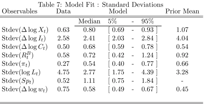
3.1 Data and Prior Selection
I estimate the model by Bayesian methods on sample that spans from 1989Q1 to 2010Q1. To
estimate the model parameters I use the following vector of eight observable time series, obtained
from Haver Analytics:
[
∆ logXt, ∆ logIt, ∆ logCt, RBt , πt, Spt, log (Lt), ∆ log
Wt
Pt
]
.
The dataset is composed of the log growth rate of real per-capita GDP,Xt=Ct+It+Gt, investment,
It, and aggregate consumption,Ct, the federal funds rate mapped into the model nominal risk-free
rate, RB
t , the GDP price deflator, πt, the spread of high-yield B-rated corporate bonds from the Merrill Lynch’s High Yield Master file versus AAA corporate yields of comparable maturity,Spt, the
log of per-capita hours worked and the growth rate of real hourly wages, Wt
Pt. Notice that I choose
the observed spread, Spt, to map into the model difference between the borrowing cost of Sellers
and the yield on risk-free government bonds, up to a measurement error ηSpt ∼N(0, σ2ηSp
)
:
Spt=Et
[
log
(
RK
t+1+ (1−δ)QAt+1
QA t
)
−RBt
]
+ηSpt
The choice of this particular series of spreads uniforms to the literature that finds high-yield spreads
to have a significant predictive content for economic activity (Gertler and Lown (1999)). In particular
these spreads are the mid-credit-quality-spectrum spreads that Gilchrist, Yankov, and Zakrajsek
(2009) find to be good predictors of unemployment and investment dynamics. The measurement
error is intended to account for the differences in the federal funds rate and the AAA corporate bond
yield, used as reference points to compute the spread in the model and the data respectively. The
measurement error is also intended to correct for the imperfect mapping of rates of return on equity
in the model onto yields on state-non-contingent bonds in the data.
Estimates for the parameters are obtained by maximizing the posterior distribution of the model
(An and Schorfheide (2007)) over the vector of observables. The posterior function combines the
model likelihood function with prior distributions imposed on model parameters and on theoretical
moments of specific variables of interest.
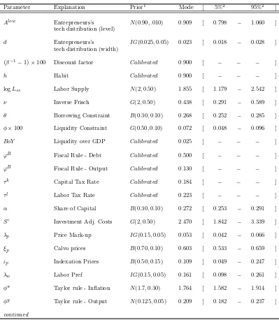
The choice of the priors for most parameters of the model is rather standard in the literature
(Del Negro, Schorfheide, Smets, and Wouters (2007), Justiniano, Primiceri, and Tambalotti (2010))
and is reported in table3.
A few words are necessary to discuss the priors selection on parameters that influence
en-trepreneurs’ investment financing decisions and the efficiency of financial intermediation in the model.
I set a Gamma prior on the steady state quarterly intermediation cost,τqss, with mean equal to 62.5
of 250 basis points chosen by C´urdia and Woodford (2010a) to match the median spread between
the Federal Reserve Board index of commercial and industrial loan rates and the federal funds rate,
over the period 1986-2007. I use my analysis of quarterly Compustat cash flow data to set the prior
mean and standard deviation on the steady state level of the financing gap share,F GS.
The aggregate of entrepreneurs in the model can easily represent the universe of corporations
in Compustat: they earn operating cash flows from their capital stock and use them to finance
new capital expenditures. They also access financial markets to either raise external financing or to
liquidate part of their assets.
Starting from the accounting cash flow identity (3) in section1, I can map its components to the
flow of funds constraint of an entrepreneur that is willing to buy and install new capital goods in
my model in section 2:
P Ce,t
| {z }
DIVe,t
+ PtKie,t
| {z }
CAP Xe,t
−
QAt φ(1−δ)Ne,t−1
| {z }
N F Ie,t
+(RBt−1Be,t−1−Be,t
) | {z }
∆CASHe,t
− θQAtAe,tie,t
| {z }
(CFD
e,t+CFe,tEO)
=RKt Ne,t−1
| {z }
CFO e,t
(31)
The returns on the equity holdings, RK
t Ne,t−1, correspond to the operating cash flows, CFOe,t. En-trepreneur’s nominal consumption, PtCe,t, can be identified with dividends paid to equity holders,
DIVe,t, and the purchase of new capital goods, PtKie,t, with capital expenditures, CAPXe,t. Net
fi-nancial operations in Compustat, NFIe,t, are mapped into net sales of old equity claims,QAtφ(1−δ) Ne,t−1, while variations in the amount of liquidity, ∆CASHe,t, correspond in the model to net
acquisitions of government bonds, (RB
t−1Bt−1−Bt). Finally transfers from debt and equity hold-ers, CFDe,t + CFEOe,t , correspond to issuances of equity claims on the new capital goods installed,
θQA
tAe,tie,t.
From (31), it is easy to derive the model equivalent of the Financing Gap Share defined in
(5). Entrepreneurs with the best technology to install capital goods (sellers) are willing to borrow
resources and to utilize their liquid assets to carry on their investment. The aggregate financing gap
over theχs,t measure of sellers, S, can be written as:
F Gt =
∫ S R K t Ns,t−1
| {z }
CFO s,t
−P Cs,t
| {z }
DIVs,t
− PtKis,t
| {z }
CAP Xs,t
f(As,t)ds
= ∫ S Q A
tφ(1−δ)Ns,t−1
| {z }
N F Is,t
+(RBt−1Bs,t−1−Bs,t)
| {z }
∆CASHs,t
− θQAt As,tis,t
| {z }
(CFD
s,t+CFs,tEO)
f(As,t)ds
= QAt
(
φ(1−δ)χs,tNt−1+
∫
S
θAs,tis,tf(As,t)ds
)
+RBt−1χs,tBs,t−1.
re-sources raised by external finance,QA
tθAs,tie,t, those raised by liquidation of selling illiquid securities,
QA
tφ(1−δ)χs,tNt−1, and from the liquid assets that come to maturity,RBt−1χs,tBt−1, over aggregate
investment,Italong the sample period:
F GSss=
QA ss
(
φ(1−δ)χs,ssNss+
∫
SθAs,ssis,ssf(As,ss)ds
)
+RB
ssχs,ssBss
Iss
.
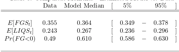
I set a Beta prior on the distribution of FGSss, with mean equal to 0.35 and standard deviation
equal to 0.01.
Similarly, I use Compustat evidence to choose a prior on the steady state share of the financing
gap that is covered by portfolio liquidations of equity claims, QA
ss(φ(1-δ)χs,ssNss), and government bonds, RB
ss χs,ss Bs,ss:
LIQSSS =
QA ss
(
φ(1−δ)χs,ssNss
)
+RB
ssχs,ssBs,ss
F Gss
.
I choose a prior the average share of the Financing Gap covered by portfolio liquidations, LIQSss,
to be a Beta distribution with mean equal to .25 and a standard deviation of .10.
I also help the identification of φ by calibrating the share of government liquidity held by
en-trepreneurs over GDP, BSS/Yt. I choose to calibrate the amount of liquid assets in circulation in
the economy by referring to the Flow of funds data on corporate asset levels (table L.102). There, I
identify a broad set of government-backed liquid assets held by firms that include Treasuries,
Cur-rency, Checking and Saving deposits, Municipal Bonds, and GSE and Agency-backed private bonds.
Along the sample considered, corporate holdings of government-backed liquid assets amounts to a
share of around 5% of GDP. I therefore fix BoY = 0.05. This is clearly and understatement of the
extent of the average amount of government-backed liquidity over GDP present in the US economy,
where the public debt over GDP alone in the same time frame amounts to an average of around
60%. I make this choice because aggregate Flow of funds data suggest that firms are not the primary
holders of government bonds and because the primary goal of this work is to offer a realistic picture
of the balance sheet and cash flow statements of US corporations to study the interaction between
financial market conditions and investment decisions.
This brings the discussion to the calibration of fiscal parameters that govern the government
budget constraint in steady state:
Bss+τkRkssKss+τlWssLss=RBssBss+
(
1− 1
gss
)
Yss+Tss (32)
To calibrate the tax rates on capital and labor income, τk and τl, I rely on work on fiscal policy
in DSGE models by Leeper, Plante, and Traum (2010). I calibrate the distortionary tax rate on
forgss to match the 19% average share of government expenditures over GDP observed during the
sample period. Having pinned down the level of government-backed liquidity, the steady state share
of lump-sum transfers to households over GDP can be found by solving (32). Transfers dynamics
instead govern the aggregate supply of liquid assets in general equilibrium over time by means of
the taxation rule:
Tt/Yt
Tss/Yss =
(
∆ logYt−s
γ
)−ϕY (B
t/Yt
BoY
)−ϕB
where I calibrate ϕB = 0.4 as in Leeper, Plante, and Traum (2010) , a value that makes this fiscal
rule passive by reducing transfers when the share of government debt over GDP deviates from its
steady state value. This locks the economy on a stable equilibrium path for the growth rate of the
price level, with no conflict with the monetary authority’s Taylor-type rule (Woodford (2003)). I fix
the elasticity of transfers to deviation of output growth from it steady state,ϕY = 0.13, at the value
that Leeper, Plante, and Traum (2010)’s estimate for transfers reactions to output deviations from
steady state in a stationary model. Notice that the transfers policy is countercyclical (when output
growth is low, transfers to households are higher).
A few more choices of priors require a brief discussion. In particular, the parameters governing
the distribution of idiosyncratic technology of entrepreneursAe,t∼U
[
Alo, Ahi]. I set priors onAlow
and on the difference d= Ahigh−Alow, so that combined with prior mean values for the financial parameters, I can approximately match the steady state share of Sellers in the model with the
average share of Compustat firms that rely on financial markets in every quarter, 45%. Finally, I
calibrate the quarterly rate of capital depreciation to 0.025, a standard value in the RBC and DSGE
literature.
The model is buffeted by i.i.d. random innovations:
[
εzt, εmpt , εgt, εpt, εwt, ετq
t , εbt
]
that respectively hit seven exogenous processes: the growth rate of total factor productivity, zt,
deviations from he Taylor ruleηmp,t, the share of government spending over GDP, gt, the price and
wage mark-ups,λptand λwt , the financial intermediation wedge,τqt and the discount factor, bt.
To conclude, the priors on the persistence parameters for the exogenous processes are all Beta
distributions. All have mean equal to 0.6 and standard deviation 0.2, except for the persistence
of the neutral technology process, ρz. The monetary policy shock is assumed to be i.i.d., because
the Taylor rule already allows for autocorrelation in the determination of the risk-free rate. The
priors on the standard deviations of the innovations expressed in percentage deviations are inverse
Gammas with mean 0.5 and standard deviation equal to 1, excluding the shock to the monetary
policy rule, εmpt , to the price and wage mark-ups,εpt and εw
t, and to the discount factor, where the