Munich Personal RePEc Archive
Data appendix for economic growth in
the long run
Tamura, Robert and Dwyer, Gerald P and Devereux, John
and Baier, Scott
Clemson University, Clemson University, Queens College, CUNY,
Clemson University
14 September 2012
Online at
https://mpra.ub.uni-muenchen.de/80768/
Data Appendix for Economic Growth in the Long Run
∗
Robert Tamura, Gerald P Dwyer, John Devereux, Scott Baier
†November 2016
Abstract
This extended data appendix describes the sources and methods used to construct the data used in our paperEconomic Growth in the Long Run.
1
Introduction
This data appendix describes the sources and procedures used to construct Figures 1-4 in the text, as well as the data for all of the empirical analyses. Almost all of the real output data come from Maddison. We used two different sources, which occasionally differ, but generally are quite similar: Maddison (1995)Monitoring the World Economy: 1820-1992, and Maddison (2003) The World Economy: Historical Statistics. All of Maddison source data is listed in 1990 Geary-Khamis dollars. We converted these into 2000 international dollars using the US GDP deflator. This keeps the data roughly consistent with our earlier work, Baier, Dwyer and Tamura (2006), except for change of base year. We generally used Maddison for all real PPP per capita income. Unless noted otherwise, all schooling data, historical age distribution data, investment data come from B. R. Mitchell (2003). I abbreviate this source as Mam, Maa, Meu forInternational Historical Statistics: the Americas, 1750-2000, International Historical Statistics: Africa, Asia and Oceania, 1750-2000, and International Historical Statistics: Europe, 1750-2000. For some population figures in 1980 and 1990 we used those from Summers and Heston online, hereafter abbreviated as S & H online. For 2000 population we used data from the Time Almanac 2001. For 2010 population we used data from
Wikipedia. The share of the population aged 15-64 for all countries in 2010 come from World Bank Development Indicators. Some age distribution data is not available from Mitchell. These are typically smaller undeveloped countries of Africa and Asia. Typically we do not have data prior to 1950. We used data from Keyfitz and Flieger (1990), which provide age distribution data in quinquennial manner from 1950-2000.
1.1
Physical Capital
Physical capital investment rates prior to 1992 were measured using Mam, Maa, and Meu. Mam, Maa and Meu provide annual information on gross physical capital formation. Between the census years t-1
∗We thank Kevin M. Murphy, Richard Rogerson, Todd Schoellman, Curtis Simon, Paula Tkac, Kei-Mu Yi for helpful
comments and suggestions. We also thank the seminar participants at the 2016 Las Vegas APEE Meetings, University of North Carolina at Chapel Hill, 2009 NBER Time and Space Conference at the Philadelphia FRB, 2009 Midwest Macroeconomics Meetings at Indiana University, Human Capital and Economic Development Conference at the Korean Labor Institute
and t, we calculate the mean investment rate. Most of the data comes from real capital formation as a fraction of real income, but when this data was missing we substituted nominal values of capital formation relative to nominal income. For some countries we used investment rates from S & H online. In order to calculate physical capital per worker, we created average investment rates over the coverage years. For example suppose we have two observations on income per worker in 1990 and 2000, respectively. In order to calculate the physical capital per worker in 2000 we use the average investment rate from 1990 to 1999 inclusive. We use a perpetual inventory method of calculation. In order to illustrate this method, assume that we observe output per worker in 1990 and 2000,y1990andy2000, respectively. Leti2000be the average
investment rate for years 1990 to 1999 inclusive, andi1990 be the investment rate in 1990. Finally assume
that k1990 is the physical capital per worker in 1990. Physical capital per worker in 1991 would be given
by:
k1991=
k1990(1−δ) +y1990i1990
gw
(1)
wheregwis the growth rate of the labor force between 1990 and 1991, andδis the annual depreciation rate
on capital. Now letgy be the annualized growth rate of output per worker from 1990 to 2000 and redefine
gw to be the annualized growth rate of labor force between 1990 and 2000. Repeated substitution of the above relation produces:
k2000=i2000y1990 9
X
i=0
(1−δ)ig9−i
y gwi+1
+(1−δ)
10k 1990
g10
w
(2)
The first term on the right hand side is, by assumption, a finite geometric sum and hence finite. The last term is an exponentially decaying term of the previous periods physical capital per worker. Thus we can rewrite the above expression as:
k2000=i2000y1990
g9 y
gw
h
1−(1−δ)
10
gygw11
i
1−(1−δ)
gygw
+(1−δ)
10k 1990
g10
w
(3)
For initial conditions we typically use information on sectoral output shares and apply the US capital -sectoral output ratios to these to construct initial capital estimates. Otherwise, we have information for other sources on the initial capital stock value.
What values of δt to use? An earlier version of this paper assumed thatδtwas a step function in the
output per worker, yt. However the work of Piketty and and Zucman (2013) convinced us that it was simpler and better to use a constant depreciation rate, independent of income. Furthermore Piketty and Zucman find that the physical capital output ratio is generally in the range of 3 or greater, whether in the 19th century, or 20th century or 21st century! For a capital output ratio of 3, a 1
30 depreciation rate would
produce a capital charge on income equal to 10% of income. We assumed for any country i:
δi=
1
30 (4)
These rates are consistent with producing k
y ratios for rich countries that are around 3 in 2010. In the final
Table 1: Regressions of PPP investment rates on nominal investment rates
variable decade average yearly observations nominal investment rate 1.6127 1.5749
(0.1017) (0.0344)
lny 0.0091 0.0093
(0.0025) (0.0009) nominal investment rate *lny -0.0838 -0.0800
(0.0127) (0.0043) constant -0.0687 -0.0697
(0.0186) (0.0065) number of observations 610 5842
¯
R2 .9065 .8989
Notes: Table reports our estimates of PPP investment PWT rates on nominal investment rates from Mitchell.
The next question is what investment rate to use. The investment rates from Mitchell are nominal investment rates. That is investment rates assuming that the price of capital is equal to the price of con-sumption for all countries. However Summers Heston provide PPP adjusted as well as nominal investment rates for countries. We ran the regression of PPP adjusted investment rates against nominal investment rates, log of real output per capita in 1985 dollars, and an interaction between nominal investment rates and log of real output per capita in 1985 dollars and a constant. However before we ran the regressions we calculated decade averages of PPP investment rates, nominal investment rates, log of real output per capita in 1985 dollars and the interaction of the average nominal investment rate and log of real output per capita in 1985 dollars. Column one of Table 1 produces these regression results. Column two of Table 1 provides a robustness check on the regressions by examining the results of a regression using all of the years of the data, instead of averaging them by decade, there are no differences. For the paper we used the results in column 1 to produce our PPP investment rates. The range of the variables are given in the following Table. The first half of Table 2 provides the mean, standard deviation, minimum and maximum for the Summers Heston 1950-2000 data. The second half of the table provides the same information for our Mitchell data. As can be seen, almost all of the values of the variables in the years prior to 1950 are completely contained in the range from 1950-2000. The notable exception is the negative investment rate in the Netherlands during the 1930s. However since this is not an initial year, it does not cause any problems in the calculations of real physical capital per worker, although obviously real capital per worker falls between 1930 and 1940! Hence our estimates of PPP investment rates are in fact projections and not extrapolations.
1.2
Sectoral Computations
Table 2: Descriptive statistics of Summers & Heston (1950-2000) and Mitchell prior to 1950
Summers & Heston 1950-2000 Mitchell prior to 1950
variable mean std dev min max mean std dev min max nominal investment rate 0.1656 0.0936 0.0121 0.5440 0.1200 0.0437 -0.008 0.3586
lny 7.852 1.025 5.658 10.134 7.364 0.644 5.623 8.755 nominal investment rate *lny 1.3532 0.8505 0.0735 4.733 0.8913 0.358 -0.0646 2.854
a century! So we have modified our approach using sectoral output shares. Typically Mitchell provides sectoral output shares of GDP, which we aggregate into three categories: farming, manufacturing and services. Manufacturing is a catch-all category that includes manufacturing, mining and construction.1 We
generally have data from 1950-2010, where for the richest countries we often have sectoral output shares back into the 19th century. In order to estimate sectoral shares where no data was found, we used Sabillon (2005). He provides decade growth rates for the 1950s, 1960s, 1970s, 1980s and 1990s, half century growth rates 1900-1950, and 19th century growth rates of GDP, agriculture and most times manufacturing and occasionally services. His coverage is almost comprehensive with our countries. In order to compute past sectoral shares we used the following typical formula:
sag,t−X =sag,texp(−X[γag,t−X−γy,t−X]) (5)
sman,t−X =sman,texp(−X[γman,t−X−γy,t−X]) (6)
sservices,t−X = 1−sag,t−X−sman,t−X (7)
where X is the number of years prior to the first observed value of sectoral output share, γag,t−X is the
annual growth rate of agriculture in the decade containing yeart−X,γy,t−X is the annual growth rate of
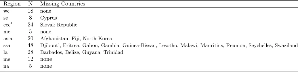
GDP in the decade containing yeart−X. When we do not have growth rate observations on say agriculture or manufacturing, for some countries, we almost always have growth rate observations on services. Below we list in Table 3 the countries that Sabillon does not have: 2 Table 4 provides the sectoral capital-output
Table 3: Missing Countries from Sabillon (2005) Sectoral Data
Region N Missing Countries
wc 18 none
se 8 Cyprus
cee1
24 Slovak Republic
nic 5 none
asia 20 Afghanistan, Fiji, North Korea
ssa 48 Djibouti, Eritrea, Gabon, Gambia, Guinea-Bissau, Lesotho, Malawi, Mauritius, Reunion, Seychelles, Swaziland la 28 Barbados, Belize, Guyana, Trinidad
me 12 none
na 5 none
1
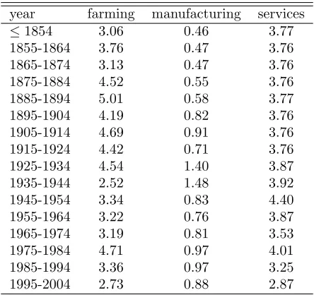
[image:5.612.72.590.549.674.2]ratios for the U.S. by time period that are used to produce aggregate capital for a country in which real investment rates are not available, and other papers have not constructed capital stock estimates. In this
Table 4: U.S. sectoral capital output ratios
year farming manufacturing services
≤1854 3.06 0.46 3.77 1855-1864 3.76 0.47 3.76 1865-1874 3.13 0.47 3.76 1875-1884 4.52 0.55 3.76 1885-1894 5.01 0.58 3.77 1895-1904 4.19 0.82 3.76 1905-1914 4.69 0.91 3.76 1915-1924 4.42 0.71 3.76 1925-1934 4.54 1.40 3.87 1935-1944 2.52 1.48 3.92 1945-1954 3.34 0.83 4.40 1955-1964 3.22 0.76 3.87 1965-1974 3.19 0.81 3.53 1975-1984 4.71 0.97 4.01 1985-1994 3.36 0.97 3.25 1995-2004 2.73 0.88 2.87
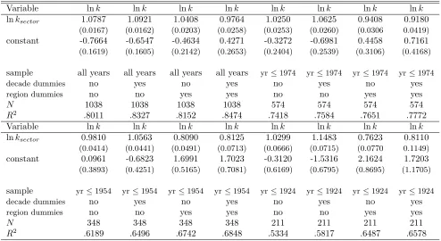
subsection we demonstrate that the physical capital stock measures derived from sectoral output shares are reasonable. There are two concerns that arise from our method of estimating physical capital using sectoral output shares. The first is that we only have sectoral physical capital - output ratios for the United States, and hence applying these to countries outside of the United States maybe problematic. The second concern is that our measure of sectoral physical capital - output ratios are only available for the United States back to 1850, and the use of the 1850 value for all years prior to 1850 maybe problematic. Here we believe that we can convince the reader that neither of these worries are too severe to prevent the use of this method. We show this by regressing the log of physical capital taken from other individuals, or from our perpetual inventory calculation against the log of physical capital per worker from the sector method. Of course when we use the sectoral method to produce the estimate, we do not include these in the regression. For all years, except 2010, we have estimates from the sectoral method. Table 5 presents the results of these regressions. We run four samples, all years, only years before 1975, only years before 1955 and only years before 1925. The samples decline from 1038 observations, to 574, 348 and 211. We include region dummies and decade dummies. The results are robust to inclusion of these region and decade controls. We find that the sectoral capital per worker estimates are highly and significantly correlated with the measures of capital per worker arising from other researchers like Piketty and Zucman, as well as by perpetual inventory. The typical coefficient on log sectoral physical capital per worker ranges from 0.76 to 1.079. Our view is that the sectoral capital stock is a good estimate of physical capital when other researchers have not produced
2
estimates of physical capital.
Table 5: Log Physical Capital per Worker Stock Regressions
Variable lnk lnk lnk lnk lnk lnk lnk lnk
lnksector 1.0787 1.0921 1.0408 0.9764 1.0250 1.0625 0.9408 0.9180 (0.0167) (0.0162) (0.0203) (0.0258) (0.0253) (0.0260) (0.0306 0.0419)
constant -0.7664 -0.6547 -0.4634 0.4271 -0.3272 -0.6981 0.4458 0.7161
(0.1619) (0.1605) (0.2142) (0.2653) (0.2404) (0.2539) (0.3106) (0.4168)
sample all years all years all years all years yr≤1974 yr≤1974 yr≤1974 yr≤1974
decade dummies no yes no yes no yes no yes
region dummies no no yes yes no no yes yes
N 1038 1038 1038 1038 574 574 574 574
R2 .8011 .8327 .8152 .8474 .7418 .7584 .7651 .7772 Variable lnk lnk lnk lnk lnk lnk lnk lnk
lnksector 0.9810 1.0563 0.8090 0.8125 1.0299 1.1483 0.7623 0.8110
(0.0414) (0.0441) (0.0491) (0.0713) (0.0666) (0.0715) (0.0770 0.1149)
constant 0.0961 -0.6823 1.6991 1.7023 -0.3120 -1.5316 2.1624 1.7203
(0.3893) (0.4251) (0.5165) (0.7081) (0.6169) (0.6795) (0.8695) (1.1705)
sample yr≤1954 yr≤1954 yr≤1954 yr≤1954 yr≤1924 yr≤1924 yr≤1924 yr≤1924
decade dummies no yes no yes no yes no yes
region dummies no no yes yes no no yes yes
N 348 348 348 348 211 211 211 211
R2 .6189 .6496 .6742 .6848 .5334 .5817 .6487 .6578
1.3
Labor Force
each country, we list explicitly these participation rates, as well as the fit of the data using this method in overlapping years.
1.4
Schooling and Human Capital
Enrollment rates for years prior to 2010 generally come from Mitchell. When reported primary and sec-ondary school enrollments are reported separately, we used the age distribution of the population 0-4, 5-9, 10-14, 15-19 to produce the relevant enrollment rates. When they are not reported separately, we typi-cally assumed that the vast majority of enrollments are primary school attendees. There is typitypi-cally an overlapping observation year, with enrollment rates reported by World Development Reports or Human Development Reports, that allow us to assign the proportion enrolled in each school category in the over-lapping years, and then gradually reduce the secondary share of total enrollments back in time. The details are given in each country description. Finally for years prior to data from Mitchell on school enrollment, we used estimates of literacy from various sources, and other estimates of enrollments, again detailed within each country’s description. Enrollment rates for 2010 come fromWorld Development Indicators. After the penultimate draft of this paper was written, we became aware of Lee & Lee (2016) in working paper form. Their original contribution produces years of schooling for men and women 15-64, from 1870-2010. They have enrollment data prior to 1870, but mostly concentrate on 1870 onward. Their work provides years of schooling estimates for 111 countries.
To calculate the stock of human capital of each type, primary school stock, secondary school stock and higher education stock, we used a perpetual inventory method. We focused on males, but we typically used information on total enrollments, not enrollments of men, as this typically is not available in Mitchell. Although this induces a downward bias in the measure of male enrollments, we feel that the information is still valuable. We used the same method as in BDT (2006), which is a variant of TTMB (2007). The following example will illustrate the nature of our calculations. In periodt+ 1, the stock of adults,Ht+1]i,
aged 25 and older, with exposure to education leveli, i=none, primary (but no more), secondary (but no more) and higher education (but no more) is given by:
Hti+1 =Hti(1−δthc) +Iti (8)
whereδhc
t is thedeath rate andItiis the flow of new adults with exposure to education leveliand no more.
We assumed thatδhc
t does not vary by education class. It is useful to put the human capital measure as a
fraction of the labor force. Thus we normalize and produce:
Hti+1
Lt+1
=H
i t Lt
Lt Lt+1
(1−δthc) + Ii
t Lt+1
(9)
hit+1=hit Lt Lt+1
(1−δhct ) + I
i t Lt+1
(10)
used the following equation:
Lt+1=Lt(1−δhct ) +rhit ℓ[9−24]t+ (r sec
t −rhit )ℓ[8−17]t+ (r el
t −rsect )ℓ[0−13]t+ (1−r el
t)ℓ[0−13]t (11)
where rhi
t is the higher education enrollment rate, rsect is the secondary school enrollment rate, relt is the
primary school enrollment rate, andℓ[i−jt] is the number of males between the ages of i and j, inclusive in period t. Notice that this definition allows for the calculation of the common term in all equations,
Lt
Lt+1(1−δ
hc
t ) in terms of obsevables:
Lt Lt+1
(1−δthc) = 1−rhit ℓ[9−24]t−(rtsec−rhit )ℓ[8−17]t−(rtel−rtsec)ℓ[0−13]t−(1−relt)ℓ[0−13]t (12)
To complete the analysis we use the information on enrollments for Ii
t. In this example, these are:
Ithi=rhit ℓ[9−24]t (13)
Itsec= (rtsec−rhit )ℓ[8−17]t (14)
Itel = (relt −rsect )ℓ[0−13]t (15)
Itnone= (1−rtel)ℓ[0−13]t (16)
1.5
Extent of Data Imputation
In this section we detail the degree of data imputation. We believe that the level of imputation is small, arguably less than 5 percent of the observations, and insignificant. We do not impute real output. So all imputed data occur in order to use the data on output per worker. Population is never imputed for any country. Data for the age distribution, labor force, education enrollments and investment rates are possible candidates for imputation. Our main concern is with schooling data.
We supplement the MitchellHistorical Statisticsvolumes with data fromWorld Development Indicators,
WDI for 2000 and 2010 when needed. For historical data prior to Mitchell, we used a variety of sources, each country entry details these. The most important data sources were Benavot & Riddle (1988), Morrisson & Murtin (2009) and Easterlin (1981, 1998). When our early values are able to match the 1870 stock education shares of Morrisson & Murtin, we consider the information validated.3 As a result, out of 2044
observations only 85 primary school enrollment rates were extrapolated. In addition to these sources we used information on literacy contained in: Morris and Adelman (1988), Steckel and Floud (1997), and Benavot and Riddle (1988). We follow the rule that it takes 3 years of schooling to become literate, see Harman (1970), Mitch (1984,2004) and Resnick and Resnick (1977). Out of 168 countries only 12 countries have extrapolated primary school enrollment rates. Of these 12, 9 have multiple years of extrapolation, three of these only extrapolate the first two or three observation years, and three more extrapolate the first observation. Thus only six countries have primary school enrollment rates that are extrapolated for more than three observations: Hong Kong (1820-1880), Nepal (1820-1900), Vietnam (1820-1890), Venezuela (1820-1880), Jordan (1820-1890), and Lebanon (1820-1890).
For secondary school enrollment rates, 6.5 percent of the observations are extrapolated, 133 out of 2044. Here 18 countries out of 55 countries inWestern Countries,Southern Europe,Central & Eastern Europeand
3
Newly Industrialized Countrieshave extrapolated values for secondary school enrollments. These countries are responsible for 78 out of 133 extrapolated values. Typically these are the earliest observations, and even more than with primary school enrollment rates, the first observations from data are typically very small values. In Asia only 6 out of 20 countries have extrapolated values. Sub-Saharan Africa has only 1 out of 48 countries requiring data extrapolation. Only 1 out of 28Latin America countries have extrapolated values, Argentina (1800-1860). Four out of 12 Middle East countries have extrapolated values. Jordan (1820-1890), Lebanon (1820-1890) are 16 of the 19 extrapolated values. Morrison & Murtin do not provide any education measures for Jordan and Lebanon. North Africa did not have any extrapolated values.
For higher education enrollment rates, only 109 of the 2044 observations are extrapolated. Two of 18 countries in the Western Countries region have extrapolated values, but only 3 observations out of 355 are extrapolated. All but one of these are first observations, and the other is a second observation. No extrapolated observations come from the Southern Europe region. Four of 28 countries in Central & Eastern Europe have extrapolated values. The Czech Republic (1820-1900), Poland (1870-1910) and Romania (1870-1890) are responsible for 17 out of 18 extrapolated values. None of these countries are in Morrisson & Murtin database, and thus cannot be benchmarked. In the Newly Industrialized Countries
region Hong Kong (1820-1940), Singapore (1820-1870) and Taiwan (1820-1905) are the countries that have extrapolated values. As with the Central & Eastern Europe region, none of these countries are in the Morrisson & Murtin database. They constitute 29 extrapolated observations. Thus Three of the 20 countries in Asia have extrapolated values. However only Nepal (1820-1900) and Vietnam (1820-1890) have extrapolated observations other than first observations. These two countries are not in the Morrisson & Murtin database. They are 17 of the 18 extrapolated values. Of the 48Sub-Saharan Africacountries, 11 have extrapolated values. However only Namibia has extrapolated values that are not first observations. Only 2 of 373 observations from Latin America are extrapolated, and only 2 out of 28 countries have extrapolated values. In theMiddle East region 5 of 12 countries have extrapolated values. Three of these five countries have extrapolated first or second observations. Only Jordan 1910) and Lebanon (1820-1930) have extrapolated values for observations beyond the first or second year. As before, we have missing values because these two countries are not in the Morrisson & Murtin database. FinallyNorth Africa has no extrapolated values.
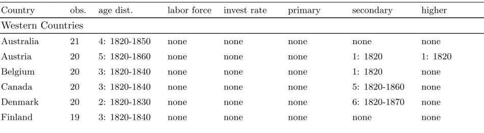
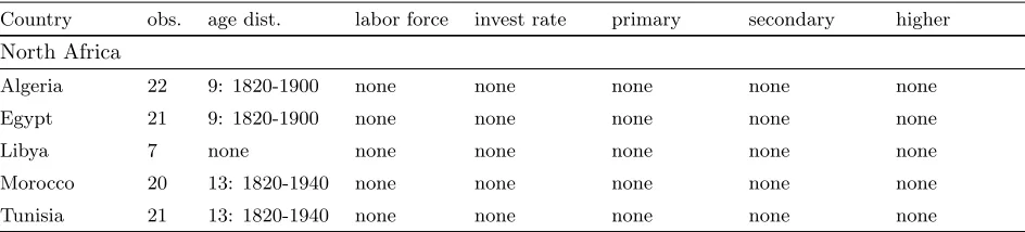
[image:10.612.77.552.614.745.2]Thus for the schooling data, we have at most 181 observations with extrapolated values. Hence less than 9% of the observations required extrapolations in schooling. Typically these are first observations, where schooling enrollment rates are typically very low and we benchmark the observation with the closest data point from the country.
Table 6: Data Imputation: Non Interpolated Values
Country obs. age dist. labor force invest rate primary secondary higher
Western Countries
Australia 21 4: 1820-1850 none none none none none
Austria 20 5: 1820-1860 none none none 1: 1820 1: 1820
Belgium 20 3: 1820-1840 none none none 1: 1820 none
Canada 20 3: 1820-1840 none none none 5: 1820-1860 none
Denmark 20 2: 1820-1830 none none none 6: 1820-1870 none
Country obs. age dist. labor force invest rate primary secondary higher
France 24 5: 1800-1840 none none none none none
Germany 23 7: 1800-1860 none none none 3: 1800-1820 none
Iceland 7 none none none none none none
Ireland 20 4: 1820-1850 none none none 5: 1820-1860 none
Luxembourg 7 none none none none none none
Netherlands 22 4: 1800-1830 none none none 4: 1800-1830 2: 1800-1810
New Zealand 25 5: 1820-1860 none none none 6: 1820-1874 none
Norway 20 3: 1820-1840 none none none 2: 1820-1830 none
Sweden 22 none none none none none none
Switzerland 20 5: 1820-1860 none none 1: 1820 1: 1820 none
UK 22 2: 1801-1811 none none none none none
USA 23 1: 1790 none none none none none
Southern Europe
Cyprus 7 none none none none none none
Greece 20 5: 1820-1860 none none none none none
Israel 8 none none none none none none
Italy 20 4: 1820-1850 none none none none none
Malta 6 none none none none none none
Portugal 22 6: 1800-1849 none none none none none
Spain 22 5: 1800-1840 none none none 5: 1800-1840 none
Turkey 21 12: 1820-1927 none none none none none
Central and Eastern Europe
Albania 15 8: 1870-1940 none none none none none
Armenia 5 none none none none none none
Azerbaijan 5 none none none none none none
Belarus 5 none none none none none none
Bulgaria 16 2: 1870-1880 none none none 1: 1870 none
Czech 20 9: 1820-1900 none none none none 9: 1820-1900
E Germany 5 none none none none none none
Estonia 5 none none none none 1: 1970 1: 1970
Georgia 5 none none none none none none
Hungary 15 none none none none none none
Kazakhstan 5 none none none none none none
Kyrgyzstan 5 none none none none none none
Latvia 5 none none none none none none
Lithuania 5 none none none none none none
Moldova 5 none none none none none none
Poland 15 5: 1870-1910 none none none 5: 1870-1910 5: 1870-1910
Romania 16 3: 1870-1890 none none none none 3: 1870-1890
Russia 20 8: 1820-1890 none none none 3: 1820-1840 none
Country obs. age dist. labor force invest rate primary secondary higher
Tajikistan 5 none none none none none none
Turkmenistan 5 none none none none none none
Ukraine 5 none none none none none none
Uzbekistan 5 none none none none none none
Yugoslavia 11 1: 1910 none none none none none
Newly Industrialized Countries
Hong Kong 20 13: 1820-1940 none none 7: 1820-1880 13: 1820-1940 13: 1820-1940
Japan 22 9: 1800-1880 none none none none none
Singapore 21 13: 1820-1940 none none none 6: 1820-1870 6: 1820-1870
S. Korea 21 11: 1820-1920 none none none none none
Taiwan 22 8: 1820-1890 none none none 10: 1820-1905 10: 1820-1905
Asia
Afghanistan 7 none none none none none none
Bangladesh 7 none none none none none none
Bhutan 4 none none none none none none
Cambodia 7 none none none none none none
China 20 13: 1820-1940 none none 3: 1820-1840 3: 1820-1840 none
Fiji 7 none none 1: 1950 none none none
India 20 6: 1820-1870 none none 3: 1820-1840 3: 1820-1840 none
Indonesia 20 13: 1820-1940 none none none none none
Laos 7 none none none none none none
Malaysia 20 11: 1820-1920 none none none 4: 1820-1850 none
Mongolia 7 none none none none none none
Myanmar 20 6: 1820-1870 none none none none none
Nepal 20 13: 1820-1940 none none 9: 1820-1900 9: 1820-1900 9: 1820-1900
N. Korea 20 13: 1820-1940 none none none none none
Pakistan 7 none none none none none none
P. N. Guinea 6 1: 2010 none none none none none
Philippines 21 10: 1820-1913 none none none none none
Sri Lanka 21 9: 1820-1900 none none 1: 1820 1: 1820 1:1820
Thailand 20 9: 1820-1900 none none none none none
Vietnam 20 13: 1820-1940 none none 8: 1820-1890 8: 1820-1890 8: 1820-1890
Sub-Saharan Africa
Angola 7 1: 2010 none none none none none
Benin 7 none none none none none none
Botswana 7 none none none none none none
Burkina Faso 7 none none none none none none
Burundi 7 none none none none none 1: 1950
Cameroon 7 none none none none none none
Cape Verde 7 none none 2: 1950-1960 none none 1: 1950
Country obs. age dist. labor force invest rate primary secondary higher
Chad 7 1: 2010 none none none none none
Comoros 7 1: 2010 none 2: 1950-1960 1: 1950 1: 1950 1: 1950
Congo 7 none none none none none none
Cote d’Ivoire 7 1: 2010 none none none none none
Djibouti 7 2: 2000-2010 none 3: 1950-1970 none none 1: 1950
Eq. Guinea 7 1: 2010 none none none none 1: 1950
Eritrea 3 none none none none none 1: 1990
Ethiopia 7 none none none none none none
Gabon 7 1: 2010 none 1: 1950 none none none
Gambia 7 1: 2010 none 2: 1950-1960 none none 1: 1950
Ghana 15 8: 1870-1940 none none none none none
Guinea 7 none none none none none 1: 1950
G.-Bissau 7 1: 2010 none 2: 1950-1960 none none 1: 1950
Kenya 7 none none none none none none
Lesotho 7 none none 1: 1950 none none none
Liberia 7 none none none none none none
Madagascar 7 1: 2010 none none none none none
Malawi 7 none none none none none none
Mali 7 none none none none none none
Mauritania 7 none none none none none none
Mauritius 7 none none none none none none
Mozambique 7 none none none none none none
Namibia 7 none none none none none 3: 1960-1980
Niger 7 none none none none none none
Nigeria 7 none none none none none none
Reunion 7 none none 2: 1950-1960 none none none
Rwanda 7 none none none none none 1: 1950
Senegal 7 none none none none none none
Seychelles 7 none none 2: 1950-1960 none none none
Sierra Leone 7 none none none none none none
Somalia 7 1: 2010 none 1: 1950 none none none
South Africa 23 11: 1800-1900 none none none none none
Sudan 7 1: 2010 none none none none none
Swaziland 7 none none 2: 1950-1960 none none none
Tanzania 7 none none none none none none
Togo 7 none none none none none none
Uganda 7 none none none none none none
Zaire 7 1: 2010 none none none none none
Zambia 7 none none none none none none
Zimbabwe 7 1: 1950 none none none none none
Country obs. age dist. labor force invest rate primary secondary higher
Argentina 22 9: 1800-1880 none none none 7: 1800-1860 none
Bahamas 7 1: 1950 none none none none none
Barbados 7 none none none none none none
Belize 7 none none none none none none
Bolivia 15 7: 1880-1940 none none none none none
Brazil 22 7: 1800-1860 none none none none none
Chile 22 10: 1800-1890 none none none none none
Colombia 22 3: 1890-1908 none none none none 1: 1890
Costa Rica 10 none none none none none none
Cuba 22 14: 1800-1930 none none none none none
Dom. Rep. 7 none none none none none none
Ecuador 15 8: 1870-1940 none none none none none
El Salvador 10 1: 1920 none none none none none
Guatemala 10 none none none none none none
Guyana 7 none none none none none none
Haiti 8 1: 1940 none none none none 1: 1940
Honduras 10 1: 1920 none none none none none
Jamaica 20 6: 1820-1870 none none none none none
Mexico 22 10: 1800-1890 none none none none none
Nicaragua 13 none none none none none none
Panama 8 none none none none none none
Paraguay 8 none none none none none none
Peru 12 none none none none none none
Puerto Rico 7 none none none none none none
Suriname 7 none none 1: 1950 none none none
Trinidad 7 none none none none none none
Uruguay 23 9: 1800-1890 none none none none none
Venezuela 23 14: 1800-1928 none none 7: 1820-1880 none none
Middle East
Bahrain 7 none none none none none 1: 1950
Iran 21 13: 1820-1940 none none none none none
Iraq 20 13: 1820-1940 none none none none none
Jordan 20 13: 1820-1940 none none 8: 1820-1890 8: 1820-1890 10: 1820-1910
Kuwait 7 none none none none none none
Lebanon 20 13: 1820-1940 none none 8: 1820-1890 8: 1820-1890 12: 1820-1930
Oman 7 none none none none none none
Qatar 7 none none none none 1: 1950 1: 1950
Saudi Arabia 7 none none none none none none
Syria 20 13: 1820-1940 none none none none none
UAE 7 none none none 2: 1950-1960 2: 1950-1960 2: 1950-1960
Country obs. age dist. labor force invest rate primary secondary higher
North Africa
Algeria 22 9: 1820-1900 none none none none none
Egypt 21 9: 1820-1900 none none none none none
Libya 7 none none none none none none
Morocco 20 13: 1820-1940 none none none none none
[image:15.612.78.550.96.203.2]Tunisia 21 13: 1820-1940 none none none none none
Table 7: Extent of Data Imputation
invest schooling
Region obs. age labor rate primary secondary higher
Western Countries 355 56 0 0 1 34 3
Southern Europe 126 32 0 0 0 5 0
Central & Eastern Europe 206 36 0 0 0 10 18
N.I.C.’s 106 54 0 0 7 29 29
Asia 281 117 0 1 24 28 18
Sub-Saharan Africa 356 35 0 20 1 1 13
Latin America 373 101 0 1 7 7 2
Middle East 150 65 0 0 18 19 26
North Africa 91 44 0 0 0 0 0
World 2044 540 0 22 58 133 109
1.6
Initial Young Human Capital: 15 to 24 age group
In this section we characterize how the initial young human capital is chosen for each country, for the model with intergenerational human capital accumulation. We did not follow a strict rule, but nonetheless it can be reproduced reasonably easy with the following empirical specification. Of course all of the values of age specific human capital including initial conditions are available in the data set. Here we merely report on the general features of the initial conditions we used. Fairly simple rules are capable of reproducing the initial human capital of the youngest workers, those age 15 to 24, and all other age categories of human capital. These latter age categories are: 25 to 34, 35 to 44, 45 to 54 and 55 to 64. We present In Table 9 the empirical results, and in Table 8 the dummy variables. We present below in Table 9 two sets of results. The top panel presents the regressions of our initial log human capital of each category against fixed rule variables. The bottom panel presents the goodness of fit of the empirical model of our initial human capital conditions.
First we define some variables. Let our assumed initial, year t, human capital for 15 to 24 year olds in country i be given byh15−24
it . Construct the log relative human capital of 15 to 24 year olds in country i in
year t relative to their 15 to 24 year old counterparts in the US be:
lnrhc15−24,t
i = ln[hc
15−24
it ]−ln[hc
15−24
Compute the log of output per worker in country i in year t relative to output per worker in the US in year t as:
lnryit= ln[yit]−ln[yU St]. (18)
In both of these definitions we placed a country’s initial observation year into its respective decade. For example if we observe a country for the first time in year 1876, we place the observation in the 1880 decade and normalize by using the US value for 1880. Let T be any decade year, a year ending in zero. Then a year t lies in decade T ift∈[T−5, T + 4].
We used Schoellman (2012) to construct quality adjusted human capital measures from schooling.4 We form the relative age category human capital from schooling as:
ln Γjit=.2[Ejit−EU S,tj ]. (19)
where E is the years of schooling for country i, in cohort t, and in age categoriesj = 15−24,25−34,35−
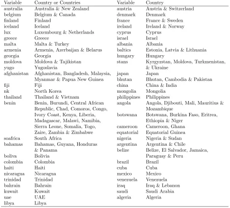
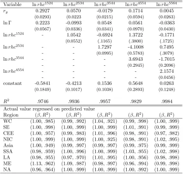
44,45−54 and 55−64. We use some country dummy variables listed in Table 8. Table 9 contains the results of the regressions of our initial relative human capital against the relative income of the country, the difference in schooling of the country’s age category with the schooling of the comparable age cohort in the US. The regressions include region dummies, and the aforementionedcountry dummies. This model does a good job of capturing our choices of initial relative human capital for all age cohorts. In all five categories the R2 exceeds .96.5 In the second panel of Table 9 we report the regression of our initial log
relative human capital against the model’s predicted log relative human capital. We report the fit of these regressions separately by region, and age category to show that the model does a good job of capturing our initial relative human capital distribution. The first term is the slope coefficient on the predicted value, and the second term is theR2of the region regression. For each age category there are 9 region results, for a total of 45 goodness of fit measures. The lowestR2value is .918, and only 3 other times is theR2 below
.950. The slope coefficient is greater than 1.02 only 4 times. It is lower than .98 only 2 times.
1.7
Special experience return values
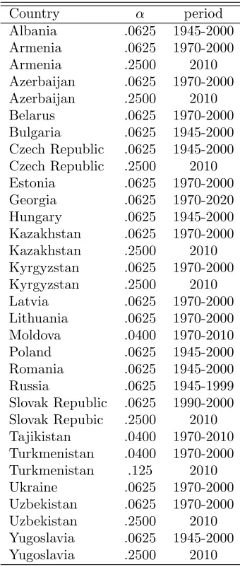
For the countries of the Central & Eastern Europe region, we used lower experience returns during their communist period. These are detailed in Table 10. The special value arises from the expression:
experience return =α∗.0495. (20)
We report the value of αin Table 10. In addition during the transition from the communist period, we removed all returns to experience during the communist period. Thus the 2000 and 2010 values of human capital are computed using only the schooling acquired during the communist period, and experience after the fall of communism in 1990. Thus in 2000, the most experience any cohort could have would be 10 years. This generally reduced human capital, but for some countries with exceptionally low returns to experience during communism, the human capital could actually rise.
4
These measures come from Schoellman (2012) and personal correspondence.
5
Table 8: Country or Region Group Dummy Variables
Variable Country or Countries Variable Country
australia Australia & New Zealand austria Austria & Switzerland belgium Belgium & Canada denmark Denmark
finland Finland france France & Sweden iceland Iceland ireland Ireland & Norway lux Luxembourg & Netherlands cyprus Cyprus
greece Greece israel Israel
malta Malta & Turkey albania Albania
armenia Armenia, Azerbaijan & Belarus baltics Estonia, Latvia & Lithuania georgia Georgia hungary Hungary
moldova Moldova & Tajikistan stans Kyrgyzstan, Moldova, Turkmenistan,
yugo Yugoslavia & Ukraine
afghanistan Afghanistan, Bangladesh, Malaysia, japan Japan
Myanmar & Papua New Guinea bhutan Bhutan, Cambodia & Pakistan fiji Fiji china China & India
nk North Korea mongolia Mongolia thailand Thailand & Vietnam philippines Philippines
benin Benin, Burundi, Central African angola Angola, Djibouti, Mali, Mauritius & Republic, Chad, Comoros, Congo, Mozambique
Ivory Coast, Kenya, Liberia, botswana Botswana, Burkina Faso, Eritrea, Madagascar, Malawi, Namibia, Ethiopia & Niger
Sierra Leone, Somalia, Togo, cameroon Cameroon, Ghana Zaire, Zambia & Zimbabwe equatorial Equatorial Guinea soafrica South Africa nigeria Nigeria & Sudan bahamas Bahamas, Guyana, Honduras argentina Argentina & Chile
& Panama belize Belize, El Salvador, Jamaica, boliva Bolivia Paraguay & Peru
colombia Colombia brazil Brazil
haiti Haiti cuba Cuba
nicaragua Nicaragua mexico Mexico trinidad Trinidad venezuela Venezuela bahrain Bahrain iraq Iraq & Lebanon kuwait Kuwait saudi Saudi Arabia
uae UAE algeria Algeria
Table 9: Log Relative Initial Young Human Capital Regressions
Variable lnrhc1524 lnrhc2534 lnrhc3544 lnrhc4554 lnrhc5564
ry 0.2927 0.0570 -0.0179 0.1714 0.0045
(0.0293) (0.0223 (0.0215) (0.0594) (0.0263)
ln Γ 0.2223 -0.0993 0.0548 0.0561 -0.0363
(0.0567) (0.0336) (0.0341) (0.0970) (0.0430)
lnrhc1524 - 1.0542 -0.6924 1.3722 -0.1771
(0.0552) (.1165) (.3800) (.1725)
lnrhc2534 - - 1.7297 -4.1008 0.7495
- - (0.0995) (0.5783) (.3079)
lnrhc3544 - - - 3.6943 -1.7015
- - - (0.2945) (0.2096)
lnrhc4554 - - - - 2.1574
- - - - (0.0456)
constant -0.5841 -0.4213 0.1536 0.5648 0.0263
(0.1849) (0.1017) (0.1038) (0.2893) (0.1248)
R2 .9746 .9936 .9957 .9829 .9984 Actual value regressed on predicted value
Table 10: Special experience returns: Central & Eastern Europe
2
Special Depreciation Rates
In this section we detail the special depreciation rates for some countries that attempt to take into account special circumstances, like the end of centrally planned communism, and exceptionally bad government institutions. We model this by introducing a special depreciation rate, ˆδ. These occur in general for the year 2000, and for a few additional countries, the year 2010.
k2000=i2000y1990
g9 y
gw
h
1−(1−δ)10
gyg11w
i
1−(1−δ)
gygw
+(1−δ)
10k 1990
g10
w
(1−ˆδ). (21)
Table 11: Special Physical Capital Depreciation Rates
country δˆ year note (rank out of 179 countries) All Central & East European Countries 12 2000 end of communism
Azerbaijan 1
7 2010 91
Belarus 17 2010 153
Bolivia 1
4 2000 & 2010 146
Congo 12 2000 & 2010 167
Cuba 1
2 2000 & 2010 177
Eritrea 12 2000 & 2010 175
East Germany 14 1990 end of communism
Iran 1
2 2000 & 2010 171
Iraq 12 2000 & 2010 N/A
Kyrgyzstan 1
7 2010 88
Lebanon 12 2000 90
Libya 207 2000 & 2010 176
Moldova 1
7 2010 124
Myanmar 12 2000 & 2010 173
North Korea 1
2 2000 & 2010 least economic freedom, 179
Sierra Leone 12 2000 & 2010 152
Russia 1
7 2010 144
Tajikistan 3
5 2010 129
Turkmenistan 17 2010 168
Ukraine 1
7 2010 163
Uzbekistan 17 2010 164
Venezuela 1
2 2000 & 2010 174
Vietnam 14 2000 & 2010 136
Zaire 12 2000 & 2010 172
Zimbabwe 1
3
Western Countries
3.1
Australia (1820-2010)
Populations for 1820, 1830, 1840, 1850, 1861, 1871, 1881, 1891, 1901, 1911, 1921, 1933, 1947, 1954, 1961, 1971, 1980, 1990 come from Maa Table A5 p. 64, 65 and 66. Population for 2000 comes fromTime Almanac 2001. Population for 2010 comes fromWikipedia.
The age distributions of the population for 1861, 1871, 1881, 1891, 1901, 1911, 1921, 1933, 1947, 1954, 1961, 1971, 1981 and 1990 come from Maa Table A2 p. 28. The age distribution for Australia in 1820, 1830, 1840, 1850 are assumed to be that of 1861. The age distribution for Australia for 1990 is interpolated from 1981 and 1992 values. The age distribution for Australia for 2000 and 2010 come from
Demographic Yearbook. For 2000 we adjusted the 2002 age distribution, and for 2010 we adjusted the 2012 age distribution. We adjust by assuming the same share by age category as in the reference year.
Labor force data for 1820 and 1830 come from Table 3.9 fromForming a Colonial Economy: Australia 1810-1850 by N. G. Butlin. Labor force data for 1840, 1850, 1861, 1871, 1881, 1891, 1901, 1911, 1921, 1931, 1951, 1961, 1971, 1981, 1991, 2000, and 2010 come from Table A2 ofThe Cambridge Economic History of Australia, edited by Simon Ville and Glenn Withers. The Table was produced by Matthew Butlin, Robert Dixon and Peter Lloyd. Male and female labor force values for 1820 and 1830 come from Butlin. We applied Butlin’s male and female shares for 1840 and 1850 to our labor force data from Butlin, Dixon and Lloyd values. For years 1861, 1871, 1881, 1891, we used the average male share of labor force for years 1840, 1850, and 1901. To compute male and female labor force values, we used information for 1901, 1911, 1921, 1931, 1941, 1951, 1961, 1971, 1980 and 1990 come from Maa Table B1 p. 102. Male and female shares of labor force for 2000 come from WDR, and male and female shares of labor force for 2010 come fromWDI.
Real GNPs come from Maddison. We convert his estimate of output per capita by multiplying by population and dividing by our estimate of labor force. For 1820, 1830, 1840, and 1850 we used the sectoral output shares from Table A1 ofThe Cambridge Economic History of Australia, edited by Simon Ville and Glenn Withers. The Table was produced by Matthew Butlin, Robert Dixon and Peter Lloyd. We then applied the sectoral capital-output ratio for the US for those years, except that we used the 1850 US values for 1820, 1830 and 1840. These formed the initial conditions for our perpetual inventory calculations beyond 1850. Physical capital investment rates come from the intraperiod average gross real capital formation and real income for 1861-1998 from Maa Table J1, pp. 1039, 1040 and 1041 and WDR (various years). For years 1971, 1981, 1991, 2000 we used the capital - output ratio from Pitketty and Zucman (2013). For 2010 we used the average investment rates from S & H online for 2000-2009, and perpetual inventory.
of students in 1881 were primary students. Seventy-five percent of students in 1891, 1901, 1911, 1921 were primary students. Seventy percent of students in 1931 were primary students. Two thirds of students in 1947, 1954 were primary students. Fifty-five percent of students in 1961 were primary students. Higher education enrollments for 1906-1998 from Maa Table I2 p. 1006. For 2010 we usedHDR. We interpolated for all enrollment rates in 2000. For years prior 1820 to 1901 we used enrollment rates of 0, 0, 0, 0, .0001, .001, .001, .001, .002. With our assumptions in the early years, we are able to match the Morrisson & Murtin education shares from 1870-1900. Our time series of years of schooling in the labor force for 1871-1921 is: 2.61 (1871), 4.13 (1881), 5.02 (1891), 5.77 (1901), 6.30 (1911) and 6.67 (1871-1921). The Morrisson & Murtin time series of years of schooling is: 3.06 (1870), 4.15 (1880), 5.28 (1890), 6.25 (1900), 7.06 (1910) and 7.71 (1920).
3.2
Austria (1820-2010)
Population figures are for the Austrian Provinces of the Hapsburg Empire, 1820, 1830, 1842, 1850, 1860, 1869, 1880, 1890, 1900 and 1910, from Meu Table A2 p. 13. Populations for Republic of Austria 1923, 1934, 1951, 1961, 1971, 1981, 1991 come from Meu Table A2 p. 13. Population for Austria 2000 comes fromTime Almanac 2001. Population for Austria 2010 comes fromWikipedia.
The age distributions of the population for 1869, 1880, 1890, 1900, 1910, 1923, 1934, 1951, 1961, 1971, 1981, 1991 come from M (1980) Table A2 p. 13. We assumed the same age distribution in 1820, 1830, 1842, 1850, 1860 as in 1869. Age distribution for Austria 2000 and 2010 come from the Demographic Yearbook. For 2000 we adjusted the 2002 age distribution, and for 2010 we adjusted the 2011 age distribution. We adjust by assuming the same share by age category as in the reference year.
Labor force figures for 1869, 1880, 1890, 1900, 1910, 1920, 1934, 1939, 1951, 1961, 1971, 1981, 1991 are from Meu Table B1 p. 145. The 1869 labor force only contains information on all workers. We assumed the female labor force in 1869 was the same proportion of the male labor force as it was in 1880. Labor force data for 2000 comeWDR. Labor force data for 2010 come fromWDI. For 1820, 1830, 1842, 1850, 1860 we used the following procedure.6 We used Clio infra for urbanization rates for 1800, 1850, 1900 and
1950, andWDI for 1960-2010. We interpolated for 1820-1840, 1860-1890, 1910-1940. We used rural 15-64 labor force participation rates of 95% for 1820-1869, 91.55% for 1880, 95% for 1890-1910, 78.62% for 1923, 52.32% for 1934, 65.1% for 1941, 84.25% for 1951, 95% for 1961-2010. We assumed urban 15-64 labor force participation rates of 80.8% for 1820-1869, 50% for 1880, 74.57% for 1890, 61.6% for 1900, 79.3% for 1910, 50% for 1923-1951, 61.14% for 1961, 53.05% for 1971, 55.7% for 1980, 51.95% for 1990, 56.13% for 2000 and 65% for 2010. We constructed the ratio of this labor force series with that from Meu, andWDR and
WDI. The root mean ratio of the overlapping years 1869-2010 is 1.000. The 1869, 1880 ratios are 1.000 and 1.000, respectively. The range of the ratios is 1.000 to 1.000.
Real GNPs come from Maddison. Sectoral output shares come from Meu Table J2 p. 929. They cover years 1910, 1923, 1934, 1951, 1961, 1971, 1980, 1990. For 2000 and 2010 we used WDI. For these years we produce capital by applying the US sectoral capital output ratios. These are used to check our calculations below. For the 1910-2000 period we used the US sectoral capital output ratios to produce estimates of aggregate physical capital. However these are not used, but serve as a check on our estimates
6
given below. For 1941 we used the 1951 sectoral shares and the sectoral growth rates for agriculture and manufacturing relative to aggregates growth rates in Sabillon p. 179. He provides growth rates for the 1950s, and separately for 1900-1949 period. For 1820, 1830, 1842, 1850, 1860, 1869, 1880, 1890, 1900 and 1910, we used the agriculture and manufacturing sectoral growth rates relative to aggregate growth rates in Sabillon p. 179 applied to the 1910 base year. He provides separate growth rates for the 19th century. We then used the sectoral capital output ratios from the US for years 1850-1860 to produce capital stock measures for these years. For 1820, 1830 and 1840 we applied the 1850 US sectoral capital output ratios. For 1869-1910 we used capital stock estimates from Max-Stephan Schulze (2007). These for the initial conditions for our perpetual inventory calculations for 1923 onward. Physical capital investment rates comes from intraperiod averages of real gross capital formation and real income for 1913-1998 from Meu Table J1 pp. 908, 914 922. For 2010 we used the average investment rate from 2000-2009 from S & H.
For 1830 we used Lindert for primary school enrollments, which produces a 9.45 percent primary en-rollment rate, which is indistinguishable from the 1842 and 1850 primary enen-rollment rates from Meu. We assumed a .5 percent enrollment rate for secondary school, and a .35 percent enrollment rate in higher education. These are in line with the .9 percent secondary enrollment rate and .4 percent higher education enrollment rate for 1842 from Meu. We assumed identical enrollment rates in 1820 as from 1830. This is consistent with the essentially constant literacy rate of birth cohorts 1801-1810, 1822-1820, 1821-1830, 1831-1840, Roser. Enrollments in primary and secondary school from 1842-1998 come from Meu Table I1 pp. 870, 873, 880 887. To calculate enrollment rates prior to 1971, we assumed 6-11 are primary school age and 12-17 are secondary school age. In 1971 we assumed that primary school lasts 8 years and secondary school lasts 4 years. Therefore 6-13 are primary school age and 14-17 are secondary school age. This switch occurred to fit with the enrollment rate data in WDR for 1980, 1990. Values for 2010 came from HDR. Higher education enrollments are from Meu Table I2 pp. 894, 895, 897, and 899. Our time series of years of schooling in the labor force for 1869-1923 is: .52 (1869), 1.47 (1880), 2.33 (1890), 3.08 (1900), 3.57 (1910) and 3.87 (1923). The Morrisson & Murtin time series of years of schooling is: 3.20 (1870), 3.44 (1880), 3.94 (1890), 4.63 (1900), 5.31 (1910) and 5.92 (1920).
3.3
Belgium (1820-2010)
Populations for 1820, 1830, 1840 1846, 1856, 1866, 1880, 1890, 1900, 1910, 1920, 1930, 1947, 1961, 1970, 1981, 1991 come from Meu Table A2 p. 14. Population for 2000 comes fromTime Almanac 2001. Popu-lation for 2010 comes fromWikipedia.
The age distributions of the population for 1846, 1856, 1866, 1880, 1890, 1900, 1910, 1920, 1930, 1947, 1961, 1970, 1981, 1991 come from Meu Table A2 p. 14. The age distribution for 1820, 1830 and 1840 are assumed to be identical to the age distribution in 1846. Age distribution for Belgium 2000 and 2010 come from theDemographic Yearbook. For 2010 we adjusted the 2011 age distribution. We adjust by assuming the same share by age category as in 2011.
Labor force figures for 1846, 1856, 1866, 1880, 1890, 1900, 1910, 1920, 1930, 1947, 1961, 1970, 1981 and 1990 are from Meu Table B1 p. 146. Labor force data for 2000 come fromWDR. Labor force data for 2010 comes from WDI. For 1820, 1830 and 1840 we used the following procedure. We used Clio infra for the urban population shares for 1800, 1850, 1900 and 1950, and WDI for 1960-2010. We assumed a rural 15-64 labor force participation rate of 88.115% for 1820-1840.7 We assumed a rural 15-64 labor force
7
participation rate of 83.22% for 1846, 89.24% for 1856, 90% for 1866-1880, 86.65% for 1890, 86.3% for 1900, 83.3% for 1910, 65.43% for 1920, 72.5% for 1930, 65.91% for 1940, 61.24% for 1947, 95% for 1961-1970, 65% for 1980-1990, 85% for 2000-2010. We assumed an urban 15-64 labor force participation rate of 50% for 1820-1856, 55% for 1866, 55.55% for 1880, 50% for 1890-1947, 55.33% for 1961, 55.59% for 1970, 50.12% for 1981, 58.32% for 1990, 64.31% for 2000 and 66.58% for 2010.8 We constructed the ratio of these labor
force values and those from Meu,WDRandWDI. The root mean ratio for overlapping years 1846-2010 is 1.000. The 1846 and 1856 values are 1.000 and 1.000, respectively. The range of the ratio is 1.000 to 1.000. Real GNP come from Maddison. Sectoral output shares for years 1947, 1961, 1970, 1980, 1990 come from Meu Table J2 p. 929. Sectoral output shares for 2000 and 2010 come from WDI. For years prior to 1947; 1820, 1830, 1840, 1846, 1856, 1866, 1880, 1890, 1900, 1910, 1920, 1930 and 1940, we used agriculture and manufacturing growth rates relative to aggregate growth rates in Sabillon p. 179. He provides these growth rates for the 1900-1949 period, and separately for the 19th century. We then applied the US sectoral capital output ratios for 1850-1940 to compute aggregate capital. For years prior to 1850, we used the 1850 US sectoral capital output ratios. Physical capital investment rates come from the intraperiod averages of real gross capital formation and real income for 1920-1998 from Meu Table J1 pp. 908, 914 922. Investment rate for 2010 is the average investment rate from 2000-2009 from S & H. For 1846-1970 we used Goldsmith (1985) to produce our capital stock estimates. From 1980-2010 we used perpetual inventory.
Enrollments in primary and secondary school from 1830-1993 come from Meu Table I1 pp. 870, 873, 880 887. We used the 1830 enrollment rates for 1820: 56.6 percent primary enrollment rate, 2.9 percent secondary enrollment rate and .1 percent higher education enrollment rate. This is consistent with the literacy rates in Belgium attained in 1800, Roser. To calculate enrollment rates, we assumed 6-11 are primary school age and 12-17 are secondary school age. Higher education enrollments are from Meu Table I2 pp. 894, 895, 897 and 899. The 2000 values fromWDR. The 2010 enrollment rates come fromHDR. Our time series of years of schooling in the labor force for 1866-1920 is: 4.68 (1866), 5.18 (1880), 4.40 (1890), 4.62 (1900), 5.18 (1910) and 5.62 (1920). The Morrisson & Murtin time series of years of schooling is: 4.27 (1870), 4.79 (1880), 5.17 (1890), 5.17 (1900), 5.33 (1910) and 5.57 (1920).
3.4
Canada (1820-2010)
Populations for 1820, 1830, 1840, 1850, 1860, 1871, 1881, 1891, 1901, 1911, 1921, 1931, 1941, 1951, 1961, 1971, 1981 and 1991 come from Mam Table A2 p. 11. Population for 2000 comes from Time Almanac 2001. Population for 2010 comes fromWikipedia.
The age distribution of the population for 1850, 1860, 1871, 1881, 1891, 1901, 1911, 1921, 1931, 1941, 1951, 1961, 1971, 1981 and 1991 come from Meu Table A2 p. 11. We used the age distribution in 1850 for 1820, 1830 and 1840. Age distribution for Canada 2000 and 2010 come from theDemographic Yearbook.
Labor force for 1871 comes from Maddison (2001) Table E-1, p.345. Labor force for 1881 comes from
Statistics Canada, and assuming a 5% unemployment rate. Labor force figures for 1891, 1901, 1911, 1921, 1931, 1951, 1961, 1971, 1981 and 1991 come from Mam Table B1 p. 102. Labor force data for 2000 come fromWDR. Labor force data for 2010 comes fromWDI. Labor force data for 1820, 1830, 1840, 1850, 1860 is produced via the following procedure. We used Bairoch and Goertz for urban-rural population shares
8
for 1820-1911, and Banks for 1921-1961, andWDR and WDI for 1971-2010. We assumed that the 15-64 rural labor force participation rate is 62.63% for 1820-1871, 59.3% for 1881, 58.4% for 1891, 57.5% for 1901, 62.5% for 1911, 61.91% for 1921, 62.5% for 1931-1961, 62.62% for 1971, 71.12% for 1980, 79.5% for 1990, 78.5% for 2000, for 78.5% for 2010. We assumed that the 15-64 urban labor force participation rate is 62.63% for 1820-1871, 50% for 1881-1901, 57.88% for 1911, 50% for 1921, 54.1% for 1931, 52.9% for 1941, 58.7% for 1951, 59.91% for 1961, 62.62% for 1971, 71.12% for 1980, 79.5% for 1990, 74.45% for 2000, 78.03% for 2010. We constructed the ratio of this labor force measure with that from Maddison,Statistics Canada, Mam,WDR andWDI. The root mean ratio for overlapping years 1871-2010 is 1.000. The ratios for 1871 and 1881 are 1.000, 1.000, respectively. The range of ratios is 1.000 to 1.000.
Real GNP for 1820, 1830, 1840, 1850, 1860, 1871, 1881, 1891, 1901, 1911, 1921, 1931, 1941, 1951, 1961, 1971, 1980, 1990, 2000, 2010 come from Maddison. Sectoral output shares for years 1921, 1931, 1941, 1951, 1961, 1971, 1980, 1990 come from come from Mam Table J2 pp. 788-789. Sectoral output shares for 2000 and 2010 come fromWDI. We used the 1925-1929 value from Mam for 1921. For all years prior to 1921, 1820, 1830, 1840, 1850, 1860, 1871, 1881, 1891, 1901 and 1911 we used the agriculture and manufacturing growth rates relative to the aggregate growth rates from Sabillon p. 147. He reports these growth rates for 1900-1949, and the 19th century separately. We then used the US sectoral capital output ratios for 1850-2000. Physical capital investment rates come from the gross real capital formation and real income for 1870, 1890, 1900, 1910 and 1920 come from Mam Table J1, pp. 762, 763. Physical capital investment rates come from the intraperiod average gross real capital formation and real income for 1926-1998 from Mam Table J1, pp. 763 and 767 andWDR (various years). We used the Piketty and Zucman (2014) estimates for 1971, 1980, 1990, 2000. For 2010 we used the average over the 2000-2009 period from S & H. Thus we used the 1860 physical capital stock from our sectoral calculations as the initial condition for our perpetual inventory calculations for years 1871-1961, inclusive, and perpetual inventory from 2000 to 2010 in order to create our 2010 value. The regression of log capital from perpetual inventory against the log capital from the sectoral calculation produces an R2 of .8853, with a slope coefficient on ln(k1985) of .897 and a
standard error of (.114). The intercept term is not significant. The sectoral capital estimates are very close to our perpetual inventory calculations.
1940-1970 period. Our time series of years of schooling in the labor force for 1871-1921 is: 4.67 (1871), 5.32 (1881), 5.67 (1891), 6.04 (1901), 6.24 (1911), 6.70 (1921). The Morrisson & Murtin times series of years of schooling is: 5.71 (1870), 6.20 (1880), 6.68 (1890), 7.10 (1900), 7.63 (1910), 8.04 (1920).
3.5
Denmark (1820-2010)
Populations for 1820, 1830, 1840, 1850, 1860, 1870, 1880, 1890, 1901, 1911, 1921, 1930, 1940, 1950, 1960, 1970, 1981 and 1990 come from Meu Table A2 p.17. Population for 2000 comes fromTime Almanac 2001. Population for 2010 comes fromWikipedia.
The age distributions of the population for 1840, 1850, 1860, 1870, 1880, 1890, 1901, 1911, 1921, 1930, 1940, 1950, 1960, 1970, 1981 and 1990 come from Meu Table A2 p. 17. We assumed the 1820 and 1830 age distributions were identical to the 1840 age distribution. Age distribution for Denmark 2000 and 2010 come from theDemographic Yearbook. For 2010 we adjusted the 2013 age distribution. We adjust by assuming the same share by age category as in 2013.
Labor force figures for 1870, 1880, 1890, 1901, 1911, 1921, 1930, 1940, 1950, 1960, 1970, 1981 and 1991 come from Meu Table B1 p. 147.9 Federico (2010) provides agricultural labor force for 1820, 1910,
1938, 2000, we used the Mitchell value for 1880.10 We interpolated these values to construct agricultural labor force for 1820-2000. We constructed the share of labor force that is agricultural for 1870-2000, and regressed this against log year. We predicted this share back to 1820, and applied it to produce our labor force values for 1820-1860. Labor force data for 2000 come fromWDR, and the labor force data for 2010 comes fromWDI.
Real GNP from 1820-2010 comes from Maddison. Sectoral output shares for Physical capital investment rates come from the intraperiod averages of gross real capital formation and real income for 1850-1998 from Meu Table J1, pp. 906, 909, 915 and 922 andWDR(various years). The 1820, 1830 and 1840 capital stock estimates come from our sectoral output shares. Mitchell provides sectoral output shares from 1820-1990, inclusive. We usedWDI for sectoral shares in 2000 and 2010. We applied the US sectoral capital output ratios in 1850 to the sectoral output shares in 1820, 1830 and 1840 to create physical capital stock estimates. From 1850 onward we used perpetual inventory methods to compute physical capital. The 2010 value is the average investment rate over 2000-2009 from S & H.
We used a 70 percent enrollment rate in primary school in 1820 and 1830, taken from the introduction of compulsory primary schooling in 1814 and approximately half were enrolled by that date, Gold (1996). We kept this value for 1840, 1850, 1860 and 1870 so as to fit the 76 percent enrollment rate in 1880 from Lindert. These rates are lower than the estimated literacy rates of 95 percent in 1850 from Morris and Adelman, and 95 percent from Morris and Adelman in 1870, and 81 percent from Crafts. This produces a primary exposure rate of 68 percent, matching Morrison & Murtin. For 1820-1870 we used 1.5 percent for secondary enrollment rates, which matches the 1880 Lindert value. Enrollments in primary and secondary school from 1893-1993 come from Meu Table I1 pp. 874, 881 and 887. To calculate enrollment rates, we assumed 6-11 are primary school age and 12-17 are secondary school age. Higher education enrollments from 1893-1993 come from Meu Table I2 pp. 895 and 897. We used .05 percent for 1850-1880 and .01 percent for 1820-1840. For 2000 enrollment rates we usedWDR. For 2010 enrollment rates we usedHDR..
9
These numbers are similar, but typically lower than the values contained in Henriksen. We chose to use Mitchell for consistency in source.
10
Our time series share of labor force exposed to higher education is consistent with Morrisson & Murtin 1870-2000, but we are low over the 1950-1970 period. Our time series for years of schooling in the labor force for 1870-1921 is: 4.26 (1870), 4.27 (1880), 4.46 (1890), 5.16 (1901), 5.57 (1911) and 6.00 (1921). The Morrisson & Murtin time series of years of schooling is: 4.69 (1870), 4.94 (1880), 5.25 (1890), 5.61 (1900), 5.96 (1910) and 6.33 (1920).
3.6
Finland (1820-2010)
Populations for 1820, 1830, 1840, 1850, 1865, 1880, 1890, 1900, 1910, 1920, 1930, 1940, 1950, 1960, 1970, 1980 and 1990 come from Meu Table A2 p. 18. Population for 2000 comes from Time Almanac 2001. Population for 2010 comes fromWikipedia.
The age distribution of the population for 1850, 1865, 1880, 1890, 1900, 1910, 1920, 1930, 1940, 1950, 1960, 1970, 1980 and 1990 come from Meu Table A2 p. 18. We assumed the age distributions for 1820, 1830 and 1840 were identical to the age distribution in 1850. Age distribution for Finland 2000 and 2010 come from theDemographic Yearbook. For 2000 we adjusted the 2002 age distribution, and for 2010 we adjusted the 2012 age distribution. We adjust by assuming the same share by age category as in the reference year. Labor force figures for 1820, 1830, 1840, 1850, 1865, 1880, 1890, 1900, 1910 and 1920 use data from Grigg (1987) on labor force in agriculture, adjusting for share of labor in agriculture. For this agricultural share we use the 1880, 1900, 1910 and 1920 agriculture share from Meu. We adjusted the 1900 figure labor force for female workers in agriculture that is 203 instead of 103 in order to better fit the time series. We interpolated for 1890. Labor force for 1930, 1940, 1950, 1960, 1970, 1980, 1990 come from Meu Table B1 p. 148. Labor force data for 2000 come fromWDR. Labor force data for 2010 comes fromWDI.
Real GNP come from Maddison. Physical capital investment rates come from the intraperiod averages of gross real capital formation and real income for 1865-1998 from Meu Table J1, pp. 906, 909, 915 and 922 andWDR(various years). For 1820, 1830, 1840, 1850 we used sectoral capital estimates. Mitchell provides sectoral output shares for 1865-1990, andWDI provides shares for 2000 and 2010. We used Sabillon (2005) to produce sectoral output shares for 1820-1850. Sabillon provides agriculture, and manufacturing growth rates along with aggregate growth rates in order to produce these estimates. We applied the US 1850 capital - sectoral output ratios for 1820, 1830, 1840 and 1850. For years beyond 1850 we used perpetual inventory methods. The 2010 value was the average investment rate from 2000-2009 from S & H.
years of schooling is: 1.45 (1870), 1.53 (1880), 1.62 (1890), 1.73 (1900), 2.00 (1910) and 2.71 (1920).
3.7
France (1800-2010)
Populations for 1800, 1810, 1820, 1830, 1840, 1850, 1861, 1872, 1881, 1891, 1901, 1911, 1921, 1931, 1946, 1954, 1962, 1968, 1975, 1980 and 1991 come from Meu Table A2, pp. 19 and 20. Population for 2000 comes fromTime Almanac 2001. Population for 2010 comes fromWikipedia.
The age distribution of the population for 1850, 1861, 1872, 1881, 1891, 1901, 1911, 1921, 1931, 1946, 1954, 1962, 1968, 1975, 1980 and 1991 come from Meu Table A2, pp. 19, 20 and 21. The age distribution for 1800, 1810, 1820, 1830, 1840 are assumed to be identical with the age distribution from 1850. Age distribution for France 2000 and 2010 come from the Demographic Yearbook. For 2000 we adjusted the 2002 age distribution, and for 2010 we adjusted the 2012 age distribution. We adjust by assuming the same share by age category as in the reference year.
Labor force data for 1861, 1872, 1881 and 1891 come from interpolations of data for 1856, 1866, 1886, 1896 from Meu Table B1, p. 149. Labor force figures for 1901, 1911, 1921, 1931, 1946, 1954, 1962, 1968, 1975, 1981 and 1991 come from Meu Table B1 p. 149. We interpolated for our 1940 value. The 1981 value comes from interpolations using the 1975, 1982 values. Labor force data for 2000 come fromWDR. The 2010 labor force comes fromWDI. For 1800-1850, we used the following procedure. We used Clio infra for urban population shares for 1800, 1850, 1900, 1950, and WDI for 1962-2010. We interpolated for urban shares 1810-1840, 1860-1890, 1910-1946. WE assumed rural 15-64 labor force participation rate of 80.495% for 1800-1850, 67.9% for 1861, 74.805% for 1872, 79.315% for 1881, 81.94% for 1891, 85% for 1901-1946, 81.28% for 1954, 85% for 1962-2010.11 We assumed an urban 15-64 labor force participation rate of 50%
for 1800-1891, 61.2% for 1901, 70.3% for 1911, 74.23% or 1921, 58.65% for 1931, 59.32% for 1940, 58.6% for 1946, 50% for 1954, 57.84% for 1962, 55.16% for 1968, 55.4% for 1975, 51.36% for 1980, 60.8% for 1991, 63.09% for 2000 and 67.5% for 2010.12 We constructed the ratio of this labor force with that from Meu,
WDR and WDI. The root mean ratio for the overlapping years 1861-2010 is 1.000. The 1861 and 1872 values are 1.000 and 1.000. The range of the ratio is 1.000 to 1.000.
Real GNP come from Maddison. For all years prior to 2010, we used Piketty and Zucman (2014) capital output ratios to produce our estimates of physical capital. For 2010 we used perpetual inventory using the investment average rate over the 2000-2009 period from S & H.
The 1800 enrollment rate for primary school comes from literacy rates from Steckel and Floud. We assumed a .5 percent enrollment rate for secondary school, and a .05 percent enrollment rate for higher education. The 1830 and 1840 enrollment rates for primary school and secondary school come from Lindert. The 1810 and 1820 enrollment rates are interpolated from the 1800 and 1830 rates. Enrollments in primary and secondary school from 1850-1998 come from Meu Table I1, pp. 870, 874, 882 and 888. To calculate enrollment rates, we assumed 6-11 are primary school age and 12-17 are secondary school age. Higher education enrollments for 1889-1993 are from Meu Table I2, pp. 895 897 and 899. We used .1 percent for 1800-1830, .2 percent for 1840-1861, .3 percent for 1869 and 1881 for higher education enrollment rates. The 2000 enrollment rates come from WDI. The enrollment rates for 2010 come from HDR.The higher education share fits the 1870-1920 shares in Morrisson & Murtin. Our time series for years of schooling in the labor force for 1869-1921 is: 4.20 (1869), 4.51 (1881), 4.73 (1891), 4.88 (1901), 4.99 (1911) and 5.10
11
Our 1800-1850 value is the average of our rural 15-64 labor force participation rates for 1861-1931).
12