Maximum norm error estimates of fourth order compact difference scheme for the nonlinear Schrödinger equation involving a quintic term

(1)

R E S E A R C H

Open Access

Maximum norm error estimates of

fourth-order compact difference scheme for

the nonlinear Schrödinger equation involving

a quintic term

Hanqing Hu

1

_{and Hanzhang Hu}

1*

*_{Correspondence:} [email protected] 1_{School of Mathematics, Jiaying}

University, Meizhou, P.R. China

Abstract

A compact ﬁnite diﬀerence (CFD) scheme is presented for the nonlinear Schrödinger equation involving a quintic term. The two discrete conservative laws are obtained. The unconditional stability and convergence in maximum norm with orderO(

τ

2₊_h4₎

are proved by using the energy method. A numerical experiment is presented to support our theoretical results.

Keywords: Schrödinger equation involving a quintic term; Compact ﬁnite diﬀerence scheme; Conservation; Convergence; Unconditional stability; The max norm

1 Introduction

The Schrödinger (NLS) equation is one of the most important equations of mathematical physics with applications in many fields [1–4] such as plasma physics, nonlinear optics, water waves, and bimolecular dynamics. There are many studies on numerical approaches, including finite difference [5–11], finite element [12–14], and polynomial approximation methods [15, 16], of the initial or initial-boundary value problems of the Schrödinger equations. We consider the initial-boundary value problem for the NLS equation involv-ing a quintic term:

i∂u ∂t +

∂2_u

∂x2 –

|u|2₊_|u|4_u₌_f₍_x_,_t₎_u ₍_x

l<x<xr, 0 <t≤T), (1.1)

u(x, 0) =u0(x) (xl<x<xr), (1.2)

u(xl,t) =u(xr,t) = 0 (0 <t≤T), (1.3)

whereu(x,t) is a complex function,f(x,t) is a real function,u0(x) is a prescribed smooth

function, andi2_{= –1.}

Computing the inner product of equation (1.1) withuand∂u

∂t and then taking the imagi-nary part and the real part, respectively, the two conservative laws are obtained as follows:

Q(t) =u2_L₂=Q(0), (1.4)

(2)

E(t) =∂u

∂x

2

L2

+

xr

xl

1 2|u|

4₊1

2|u|

6

dx=E(0) –

t

0

xr

xl

f(x,t)∂

∂t|u|

2_d_x_d_t_, _(1.5)

where · L2 is theL2norm.

Zhang et al. found that the nonconservative schemes may easily show nonlinear blow-up when studying for NLS equation, so they presented a conservative diﬀerence scheme in [11]. Moreover, extensive mathematical and numerical studies have been carried out for the NLS equations in the literature [17–28]. Zhang presented a diﬀerence scheme for the NLS equation involving a quintic term [27], and it was proved with orderO(τ2₊_h2_{). Then,}

in [28] Wang proposed a new diﬀerence scheme for NLS equation involving a quintic term and showed that convergence rates of the present scheme were of orderO(τ2₊_h4_{). Wang}

presented a compact finite difference scheme for the NLS equation in [22], which provided a new thinking on the theoretical proving of a compact difference scheme. There are lots of literature works concerning the Schrödinger equations using different treatments, but, to the best of our knowledge, there are few results of unconditional maximum norm con-vergence of compact difference scheme for NLS equations involving a quintic term. Thus, the purpose of this paper is to prove maximum norm error estimates of a fourth-order compact difference scheme for the NLS equation involving a quintic term.

The remainder of this paper is organized as follows. A fourth-order compact difference scheme is proposed in Sect.2. The discrete conservation laws of the difference scheme are discussed in Sect.3. In Sect.4, the convergence and stability for the compact difference scheme are proved. In the last section, numerical results will be discussed.

2 Some notations and compact ﬁnite difference scheme

For simplicity of exposition, some notations are ﬁrstly introduced. Thus, the following notations for diﬀerence operators are used:

δtunj = un

j –unj–1

τ , δxu

n j =

un j+1–unj

h , δx¯u n j =

un j –unj–1

h , u

n+1₂

j = un+1

j +unj

2 ,

δ2_xun_j =δxδ¯xunj = un

j–1– 2unj +unj+1

h2 , Ahu

n j =unj +

h2

12δ

2

xunj = 1 12

un_j_–1+ 10un_j +un_j₊₁,

whereh=xr–xl

J andτ= T

N are step sizes of space and time, respectively, andJ,Nare two positive integers.

For anyuuu,vvv∈Vh={vvv|vvv= (v0,v1, . . . ,vJ),v0=vJ= 0}, the inner product is deﬁned as

(uuu,vvv) =h J–1

j=1

ujv¯j.

The discrete norms ofuare deﬁned as

uuup_p=h J–1

j=1

|uj|p, δxuuu2=h J–1

j=0

|δxuj|2, uuu∞= max

1≤j≤J–1|uj|.

For simplicity, we deﬁne {Un

j} as the exact solution and{unj}as the numerical one. Let

(3)

diﬀerent values at diﬀerent occurrences. For the exact solution of the initial-boundary value problem (1.1)–(1.3), we assume that

max Un,δxUn,Un_∞

≤C. (2.1)

Now, we present the following compact ﬁnite diﬀerence scheme for problem (1.1)–(1.3):

iAhδtunj + 1 2δ

2

x

un_j+1+un_j–1 4Ahu

n+1

j

2

+un_j2un_j+1+un_j

–1 6Ahu

n+1

j

4

+un_j+12un_j2+un_j4un_j+1+un_j=Ah

fn+12u

n+1

j +unj 2

(j= 1, 2, . . . ,J– 1,n= 1, 2, . . . ,N– 1), (2.2)

un₀=un_J = 0 (n= 1, 2, . . . ,N), (2.3)

u0_J =u0(xj) (j= 1, 2, . . . ,J). (2.4)

Let

u u

un=un₀,un₁, . . . ,un_J_–1T,

uuun+12+uuun2=diagdiagdiagun₀+12+un₀2, . . . ,u_Jn_–1+12+un_J_–12.

(2.2) can be rewritten as

iMMMδtuuun+ 1 2δ

2

x

u

uun+1+uuun–1 4MMMuuu

n+12₊_u_u_un2_u_u_un+1₊_u_u_un

–1 6MMMuuu

n+14₊_u_u_un2_u_u_un+12₊_u_u_un4_u_u_un+1₊_u_u_un₌_M_M_Mfn+1₂uuun+1+uuun

2 ,

n= 1, 2, . . . ,N– 1,

where the matrixMis deﬁned by

M M M= 1

12

⎛ ⎜ ⎜ ⎜ ⎜ ⎝

10 1 0 · · · 0

1 10 1 · · · 0

. .. ... ...

0 · · · 0 1 10

⎞ ⎟ ⎟ ⎟ ⎟ ⎠

(J–1)×(J–1)

.

M

MMis a tridiagonal symmetric matrix, and there is a symmetric positive deﬁnite matrixHHH

such thatHHH=MMM–1_{. Thus, the compact ﬁnite diﬀerence scheme (}_2.2_)–(_2.4_{) can be rewritten}

as the following matrix equation:

iδtuuun+ 1 2HHHδ

2

x

u

uun+1+uuun–1 4uuu

n+12₊_u_u_un2_u_u_un+1₊_u_u_un

–1 6uuu

n+14₊_u_u_un+12_u_u_un2₊_u_u_un4_u_u_un+1₊_u_u_un₌_fffn+1₂uuun+1+uuun

2

(4)

un₀=un_J = 0 (n= 1, 2, . . . ,N), (2.6)

u0_J =u0(xj) (j= 0, 1, 2, . . . ,J). (2.7)

3 Some useful lemmas and discrete conservation laws

Lemma 3.1([29]) For any two mesh functions uuu,vvv∈Vh,there is

h J–1

j=1

δ_x2uj

¯ vj= –h

J–1

j=1

(δxuj)(δxv¯j).

Lemma 3.2([22]) For any real symmetric positive deﬁnite matrices HHH,we have

ReHHHδ2_xuuun+1+uuun,uuun+1–uuun= –RRRδxuuun+12–RRRδxuuun2

,

where RRR is obtained by the Cholesky decomposition for HHH,denoted as RRR=chol(HHH).

Theorem 3.1 The diﬀerence scheme(2.2)–(2.4)is conservative in the sense

Qn=uuun=Qn–1=· · ·=Q0, (3.1)

En₌_R_R_Rδ xuuun

2

+1 2uuu

n4

4+

1 3uuu

n6

6+h

J–1

j=1

fn–

1 2

j unj

2

=En–1+h J–1

j=1

fn–

1 2

j –f n–3₂

j u n j

2

=E0+ n

l=1

J–1

j=1

fl–

1 2

j –f l–3₂

j u n j

2

h, (3.2)

for n= 1, 2, . . . ,N,where Qnis discrete mass,Enis discrete energy.

Proof Computing the inner product of (2.2) withuuun+1+uuunand then taking the imaginary part, we obtain

I1+I2–I3–I4=I5,

where

I1=Im

iδtuuun,uuun+1+uuun

=Reδtuuun,uuun+1+uuun

=1

τuuu

n+12_–_u_u_un2_,

I2=

1 2Im

HHHδ_x2uuun+1+uuun,uuun+1+uuun= –2ImRRRδxuuun+

1 2_,_R_R_Rδ

xuuun+

1 2_{= 0,}

I3=

1 4Imuuu

n+12

+uuun2uuun+1+uuun,uuun+1+uuun= 0,

I4=

1 6Imuuu

n+14₊_u_u_un+12_u_u_un2₊_u_u_un4_u_u_un+1₊_u_u_un_,_u_u_un+1₊_u_u_un_{= 0,}

I5=

1 2Im

(5)

We can obtain

uuun+12–uuun2= 0.

Then we have

Qn=uuun=Qn–1=· · ·=Q0.

Computing the inner product of (2.2) withuuun+1–uuun, and then taking the real part, we get

I6+I7–I8–I9=I10,

where

I6=Reτ

iδtuuun,δtuuun

= 0,

I7=

1 2Re

HHHδ_x2uuun+1+uuun,uuun+1–uuun= –1 2RRRδxuuu

n+12

–RRRδxuuun

2

,

I8=

1 4Reuuu

n+12

+uuun2uuun+1+uuun,uuun+1–uuun=1 4uuu

n+14 4–uuu

n4 4

,

I9=

1 6Reuuu

n+14₊_u_u_un+12_u_u_un2₊_u_u_un4_u_u_un+1₊_u_u_un_,_u_u_un+1_–_u_u_un

=1

6uuu n+16

6–uuu

n6 6

,

I10=

1 2Re

fffn+12_u_u_un+1₊_u_u_un_,_u_u_un+1_–_u_u_un₌h

2 J–1

j=1

fn+12_un+1

j

2

–un_j2.

Let

En=RRRδxuuun2+ 1 2uuu

n4 4+

1 3uuu

n6 6+h

J–1

j=1

fn–

1 2

j unj

2

.

We can obtain

En=En–1+h J–1

j=1

fn–

1 2

j –f n–3₂

j u n j

2

.

Summing up for n, we have

En=E0+ n

l=1

J–1

j=1

fl–

1 2

j –f l–3₂

j unj

2

h.

4 Numerical analysis

To obtain the error estimate in the maximum norm, we need the following lemmas.

Lemma 4.1(Discrete Sobolev’s inequality [30]) Suppose that ujis mesh functions.Given ε≥0,there exists a constant C dependent onεsuch that

(6)

Lemma 4.2 (Gronwall’s inequality [30]) Suppose that the nonnegative mesh function {un_|_n_{= 0, 1, 2, . . . ,}_N_,_Nτ ₌_T_}_{satisﬁes the inequality}

un≤A+τ n

l=1

Bkuk,

where A and Bk(k= 1, 2, . . . ,N,Nτ =T)satisfying the inequality are nonnegative constants. Then,for any0≤n≤N,there is

un_∞≤Ae2τN_k=1Bk_,

whereτ is suﬃciently small such thatτ(max_k_=1,2,...,_NBk)≤1₂.

Lemma 4.3([22]) For any real symmetric positive deﬁnite matrices HHH,there exist two

pos-itive numbers C∗and C∗such that

C∗uuun2≤HHHuuun,uuun≤C∗uuun2.

Theorem 4.1 Suppose that|f(x,t)| ≤M1,|ft(x,t)| ≤M2,u0∈H01,then, for any n(0≤

nτ ≤T),the following estimates hold:

uuun≤C, uuun_∞≤C.

Proof From (3.1), we have

uuun≤C. (4.1)

From (3.2), we obtain

RRRδxuuun

2

+1 2uuu

n4 4+

1 3uuu

n6 6+h

J–1

j=1

fn–

1 2

j unj

2

=E0+ n

l=1

J–1

j=1

fl–

1 2

j –f l–3₂

j unj

2

h,

thus, we have

RRRδxuuun

2

≤E0+ n

l=1

J–1

j=1

fl–

1 2

j –f l–3₂

j unj

2

h–h J–1

j=1

fn–

1 2

j unj

2

.

On the one hand, from (4.1), we have

RRRδxuuun

2

≤E0+ n

l=1

J–1

j=1

fl–

1 2

j –f l–3₂

j unj

2

h–h J–1

j=1

fn–

1 2

j unj

2

≤E0+M1h

J–1

j=1

_un j

2

+h n

l=1

J–1

j=1

∂f_∂t

(j,l+θ)

·ul_j2

(7)

On the other hand, from Lemma4.3, we have

RRRδxuuun2=

H

HHδxuuun,δxuuun

≥C∗δxuuun2.

Then we see that

δxuuun≤C. (4.2)

From (4.1)–(4.2) and Lemma4.1, we obtain

uuun_∞≤C. (4.3)

Suppose that the truncation error

rrrn=rn₀,rn₁, . . . ,rn_J_–1T∈Vh,

then we have

rrrn₌_iδ tUUUn+

1 2HHHδ

2

x

U

UUn+1₊_U_U_Un_–1 4UUU

n+12₊_U_U_Un2_U_U_Un+1₊_U_U_Un

–1

6UUU

n+14₊_U_U_Un2_U_U_Un+12₊_U_U_Un4_U_U_Un+1₊_U_U_Un_–_fffn+12UUU

n+1₊_U_U_Un

2 . (4.4)

According to Taylor’s expansion, the following can be easily obtained.

Lemma 4.4 Suppose that u0(x)∈H01,u(x,t)∈C6,3,then we have

rn_j≤Oh4+τ2, (4.5)

δtrjn≤O

h4+τ2. (4.6)

Lemma 4.5 [[22]]For u={u0_,_u1_{, . . . ,}_un_,_un+1_}_{and g}₌_{_g0_,_g1_{, . . . ,}_gn–1_,_gn_}_,_{we have}

2τ

n

l=0

glδtul

≤u0

2

+τ n

l=1

ul2+un+12+g02+τ n–1

l=0

δtgl2+gn2. (4.7)

Theorem 4.2 Suppose that the conditions of Theorem4.1and Lemma4.4are satisﬁed,

then the numerical solution of scheme(2.2)–(2.4)converges to the solution of problem(1.1)–

(1.3)with order O(h4+τ2)in the discrete · ∞norm.

Proof Let

eeen=UUUn–uuun.

Subtracting (2.5) from (4.4), we obtain

rrrn=iδteeen+ 1 2HHHδ

2

x

eeen+1+eeen–1 4FFF

n_–1 6GGG

n_–_fffn+12eee

n+1₊_eeen

(8)

where

F F

Fn=UUUn+12+UUUn2UUUn+1+UUUn–uuun+12+uuun2uuun+1+uuun,

G G

Gn=UUUn+14+UUUn+12UUUn2+UUUn4UUUn+1+UUUn

–uuun+14+uuun+12uuun2+uuun4uuun+1+uuun,

F F

Fn=UUUn+12+UUUn2UUUn+1+UUUn–uuun+12+uuun2uuun+1+uuun

=UUUn+12+UUUn2–uuun+12+uuun2UUUn+1+UUUn

+uuun+12+uuun2eeen+1+eeen

=UUUn+1eee¯n+1+eeen+1UUU¯n+1+UUUneee¯n+eeenUUU¯nUUUn+1+UUUn+uuun+12

+uuun2eeen+1+eeen.

(4.9)

Noting thatF₀n=F_Jn= 0, from (2.1), (4.9), and Theorem4.1, we have

FFFn2≤Ceeen2+eeen+12. (4.10)

Similarly, we obtain

δxFFFn2≤Ceeen2+eeen+12+δxeeen2+δxeeen+12

, (4.11)

G G

Gn=UUUn+14+UUUn+12UUUn2+UUUn4UUUn+1+UUUn

–uuun+14+uuun+12uuun2+uuun4uuun+1+uuun

=UUUn+14+UUUn+12UUUn2+UUUn4–uuun+14+uuun+12uuun2+uuun4

×UUUn+1+UUUn

+uuun+14+uuun+12uuun2+uuun4eeen+1+eeen

=UUUn+12+UUUn+12UUUn+1eee¯n+1+eeen+1UUU¯n+1+UUUn2+UUUn2UUUneee¯n+eeenUUU¯n

+uuun2UUUn+1eee¯n+1+eeen+1uuu¯n+1+uuun+12UUUneee¯n+eeenuuu¯nUUUn+1+UUUn

+uuun+14+uuun+12uuun2+uuun4eeen+1+eeen. (4.12)

GGGn2≤Ceeen2+eeen+12, (4.13)

δxGGGn

2

≤Ceeen2+eeen+12+δxeeen

2

+δxeeen+1

2

. (4.14)

Computing the inner product of (4.9) withen+1₊_en_{and taking the imaginary part, we have}

Imrrrn,eeen+eeen+1

=Imiδteeen,eeen+eeen+1

+ImHHHδ2_xeeen+eeen+1,eeen+eeen+1–1 2Im

FFFn,eeen+eeen+1

–1

3Im

G G

Gn,eeen+eeen+1–1 2Im

(9)

For each term on the right-hand side of (4.15), we bound them as follows:

Imiδteeen,eeen+eeen+1

=1

τeee

n+12_–_eeen2_. _(4.16)

As to the second term

ImHHHδ2_xeeen+eeen+1,eeen+eeen+1= 4ImRRRδxeeen+

1

2_,_RR_Rδ_x_eeen+12_{= 0.} _(4.17)

For the last three terms on the right-hand side of (4.15), by using the Cauchy–Schwarz inequality, we obtain

1₂ImFFFn,eeen+eeen+1≤1

4

F FFn2+1

2eee n2

+eeen+12

≤Ceeen2+eeen+12, (4.18)

1₃ImGGGn,eeen+eeen+1≤1

6

G GGn2+1

2eee

n2₊_eeen+12

≤Ceeen2+eeen+12, (4.19)

1 2Im

fffn+12_eeen₊_eeen+1_,_eeen₊_eeen+1≤_C_eeen2₊_eeen+12_. _(4.20)

For the term on the left-hand side of (4.15), we have

Imrrrn,eeen+eeen+1≤1

2

rrrn2+1 2eee

n2

+eeen+12. (4.21)

From (4.15)–(4.21), we can obtain

eeen+12–eeen2≤τrrrn2+Cτeeen2+eeen+12. (4.22)

Summing (4.22) up forn, we have

_eeen2_≤_O_h4₊_τ22₊_Cτ

n

l=1

_eeel2₊_eeel+12_. _(4.23)

Whenτis small enough, it follows from Lemma4.2that

eeen≤Oh4+τ2. (4.24)

Computing the inner product of (4.8) withδteeenand taking the real part, we have

Rerrrn,δteeen

=Reiδteeen,δteeen

+1 2Re

H

HHδ_x2eeen+eeen+1,δteeen

–1

4Re

FFFn,δteeen

–1 6Re

G GGn,δteeen

–1

2Re

fffn+12_eeen₊_eeen+1_,_δ

teeen

. (4.25)

For each term on the right-hand side of (4.25), we bound them as follows:

Reiδteeen,δteeen

(10)

For the second term, it follows from Lemma3.1that 1 2Re H H

Hδ2_xeeen+eeen+1,δteeen

=–1

2τRRRδxeee

n+12_–_R_R_Rδ

xeeen

2

. (4.27)

As to the third term, it follows from (4.8) that

δteeen=i 1 2HHHδ

2

x

eeen+1+eeen– i 4FFF

n_– i 6GGG

n_–_ifffn+1₂eeen+1+eeen

2 –irrr

n_. _(4.28)

By using the Cauchy–Schwarz inequality, we obtain

ReFFFn,δteeen

=1

2Re

FFFn,iHHHδ_x2eeen+1+eeen– i 4FFF

n_– i 6GGG

n_–_ifffn+1₂eeen+1+eeen

2 –irrr

n

=–1

2 Im

FFFn,HHHδ2_xeeen+1+eeen+1 6Im

FFFn,GGGn

+Im

F F Fn,fffn+12eee

n+1₊_eeen 2

+ImFFFn,rrrn

=1

2Im

RRRδxFFFn,RRRδx

eeen+1+eeen+1 6Im

FFFn,GGGn

+Im

F F Fn,fffn+12eee

n+1₊_eeen 2

+ImFFFn,rrrn, (4.29)

where

ImRRRδxFFFn,RRRδx

eeen+1+eeen

≤1

2

R RRδxFFFn

2

+1

2RRRδxeee

n+12₊_R_R_Rδ

xeeen

2

≤C1δxFFFn2+δxeeen+12+δxeeen2

≤Ceeen+12+eeen2+RRRδxeeen+12+RRRδxeeen2

, Im F F Fn,fffn+12eee

n+1₊_eeen 2 ≤1 2 F

FFn2+M1 2 eee

n+12₊_eeen2

≤Ceeen+12+eeen2,

ImFFFn,rrrn≤1

2FFF n2

+rrrn2≤Ceeen+12+eeen2+rrrn2,

ImFFFn,GGGn≤1

2FFF n2

+GGGn2≤Ceeen+12+eeen2.

Then we have

ReFFFn,δteeen

≤Ceeen+12+eeen2+rrrn2+RRRδxeeen+1

2

+RRRδxeeen

2

. (4.30)

ReGGGn,δteeen

2

+RRRδxeeen

2

(11)

Re

fffn+12eee

n+1₊_eeen 2 ,δteee

n

2

+RRRδxeeen

2

. (4.32)

From (4.25)–(4.32), we can obtain

RRRδxeeen+1

2

–RRRδxeeen

2

≤τCτRRRδxeeen2+RRRδxeeen+12

) +Rerrrn,δteeen

+τOh4+τ22. (4.33)

Summing (4.33) up forn, we obtain

eeen2≤CτOh4+τ22+Cτ n

l=1

_RRRδxeeel

2

+RRRδxeeel+1

2

)

+Cτ n

l=1

Rerrrl_,_δ teeel

. (4.34)

From Lemma4.4and Lemma4.5, we have

τRe

n

l=1

Rerrrl,δteeel

≤

Oh4+τ22. (4.35)

Substituting (4.35) into (4.34) and applying the discrete Gronwall inequality when taking

τ suﬃciently small, we have

RRRδxeeen≤

Oh4+τ2. (4.36)

Then, from Lemma4.3, we have

δxeeen≤

Oh4+τ2. (4.37)

From (4.2) and (4.34), and using Lemma4.1, we have

eeen_∞≤Oh4+τ2. (4.38)

Similarly, we can prove the stability of the diﬀerence solution.

Theorem 4.3 Under the conditions of Theorem4.2,the solution of the diﬀerence scheme

(2.2)–(2.4)is unconditionally stable for initial data in the · ∞norm.

5 Numerical experiment

In this section, we consider the following problem:

i∂u ∂t +

∂2_u

∂x2 –

|u|2+|u|4u

(12)

u(x, 0) =e–x2+ix (–15 <x< 15), (5.2)

u(–15,t) =u(15,t) = 0 (0 <t≤1). (5.3)

An exact solution is given by

u(x,t) =e–(x–2t)2+i(x–3t). (5.4)

For problems (5.1)–(5.3), we have the following CFD scheme:

i τAh

un_j+1–un_j+1 2δ

2

x

un_j+1+un_j–1 4Ahu

n+1

j

2

+un_j2un_j+1+un_j

–1 6Ahu

n+1

j

4

+un_j+12un_j2+un_j4un_j+1+un_j=Ah

fn+12u

n+1

j +unj 2

(j= 1, 2, . . . ,J– 1,n= 1, 2, . . . ,N– 1), (5.5)

un₀=un_J = 0 (n= 1, 2, . . . ,N), (5.6)

u0_J =u0(xj) (j= 1, 2, . . . ,J). (5.7)

In order to obtain the numerical solutionun+1

j , an iterative algorithm can be used. We deﬁne the following iterative algorithm:

A_jn_–1+1(s)u_jn_–1+1(s+1)+Bn_j+1(s)u_jn+1(s+1)+Cn_j₊₁+1(s)un_j₊₁+1(s+1)=Dn_j+1(s), (5.8)

wheresdenotes the number of iteration, and

An_j_–1+1(s)= i 12+

r

2–

τ

48E n+1(s)

j–1 –

τ

72F n+1(s)

j–1 –

τ

24f n+1₂

j–1 ,

C_jn₊₁+1(s)= i 12+

r

2–

τ

48E n+1(s)

j+1 –

τ

72F n+1(s)

j+1 –

τ

24f n+1₂

j+1 ,

Bn_j+1(s)=5i 6 –r–

5τ

24E n+1(s)

j –

5τ

36F n+1(s)

j –

5τ

12f n+12

j ,

Dn_j+1(s)=

i 12– r 2+ τ 48E n+1(s)

j–1 +

τ

72F n+1(s)

j–1 +

τ

24f n+1₂

j–1

un_j_–1

+

5i

6 +r+ 5τ

24E n+1(s)

j +

5τ

36F n+1(s)

j +

5τ

12f n+1₂

j

un_j

+ i 12– r 2+ τ 48E n+1(s)

j+1 +

τ

72F n+1(s)

j+1 +

τ

24f n+1₂

j+1

un_j₊₁.

The initial value of iterationun_j+1(0)=un

j, whenun+1(s+1)–un+1(s)∞≤ε, it is the end of iteration (this paper hasε= 10–6_).

In order to compare the eﬃciency of CFD scheme with reference to the scheme in [27,

28], we give their schemes

iδˆtunj + 1 2δ

2

x

un_j+1+un_j–1–1 2u

n j

2

un_j+1+un_j–1

–1

6u

n+1

j

4

(13)

=

fnu n+1

j +unj–1 2

(j= 1, 2, . . . ,J– 1,n= 1, 2, . . . ,N– 1),

iδtunj + 1 24

–δ_x2un_j_–1+1+ 14δ2_xun_j+1–δ_x2un_j₊₁+1+–δ_x2un_j_–1+ 14δ_x2un_j –δ_x2un_j₊₁

–1

4u n+1

j

2

+un_j2u_jn+1+un_j–1

6u

n+1

j

4

+un_j+12un_j2+un_j4un_j+1+un_j

=

fn+12

un+1

j +unj 2

,

(j= 1, 2, . . . ,J– 1,n= 1, 2, . . . ,N– 1).

For convenience, we denote the one in [27] as Scheme 2, and the one in [28] as Scheme 3, respectively.

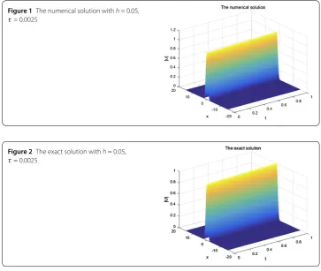
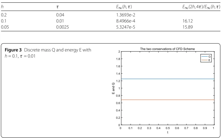
From Fig.1and Fig.2, we can see that the numerical solution of the compact scheme

and the exact solution are in good agreement. As shown in Table1, the accuracy of CFD

Scheme is higher than that of the other schemes. As indicated in Table2, the CPU time of CFD Scheme has the same CPU time cost as that of Scheme 2 and Scheme 3 in

[image:13.595.136.471.81.218.2]

computa-Figure 1The numerical solution withh= 0.05, τ= 0.0025

Figure 2The exact solution withh= 0.05, τ= 0.0025

Table 1 Comparison of the accuracy for the numerical solutions

t CFD Scheme Scheme 2 Scheme 3

0.2 3.1712e-4 4.8000e-3 3.5170e-4

0.4 6.0713e-4 8.2000e-3 6.5370e-4

0.6 7.9096e-4 1.1300e-2 8.5260e-4

0.8 8.4966e-4 1.2700e-2 9.1910e-4

[image:13.595.115.479.330.637.2] [image:13.595.114.477.664.732.2]

(14)

[image:14.595.116.480.96.144.2]

Table 2 CPU time of the three schemes

h t CFD Scheme Scheme 2 Scheme 3

0.2 0.04 0.80 s 0.81 s 0.58 s

0.1 0.01 5.83 s 6.49 s 6.23 s

0.05 0.0025 62.21 s 64.05 s 40.79 s

Table 3 Errors and convergence order at diﬀerence steps

h τ E_∞(h,τ) E_∞(2h, 4τ)/E_∞(h,τ)

0.2 0.04 1.3693e-2

0.1 0.01 8.4966e-4 16.12

[image:14.595.116.480.173.399.2]

0.05 0.0025 5.3247e-5 15.89

Figure 3Discrete mass Q and energy E with

h= 0.1,τ= 0.01

tion. From Table3, it is obvious that CFD Scheme is convergent in maximum norm, and

the convergence order isO(h4₊_τ2_{). Figure}₃_{indicates that the two conservations of CFD}

Scheme are very good.

6 Conclusion

In this paper, a compact finite difference scheme is constructed for the nonlinear Schrödinger equation involving a quintic term. The discrete maximum norm error es-timates show that the proposed schemes are in second and fourth order accurate in time and space, respectively. In numerical experiment, numerical results are carried out to confirm the theoretical analysis.

Funding

This work is supported by the National Science Foundation of China (11671157).

Competing interests

The authors declare that they have no competing interests.

Authors’ contributions

All authors contributed equally to this work. All authors read and approved the ﬁnal manuscript.

Publisher’s Note

Springer Nature remains neutral with regard to jurisdictional claims in published maps and institutional aﬃliations.

Received: 16 February 2018 Accepted: 12 July 2018 References

(15)

2. Dodd, R.K., Eilbeck, J.C., Gibbon, J.D., Morris, H.C.: Solitons and Nonlinear Wave Equations. Academic Press, New York (1982)

3. Hasegawa, A.: Optical Solitons in Fibers. Springer, Berlin (1989)

4. Sulem, C., Sulem, P.L.: The Nonlinear Schrödinger Equation Self-Focusing and Wave Collapse. Springer, New York (1999)

5. Chang, Q., Jia, E., Sun, W.: Diﬀerence schemes for solving the generalized nonlinear Schrödinger equation. J. Comput. Phys.148(2), 397–415 (1999)

6. Dai, W.Z.: An unconditionally stable three-level explicit diﬀerence scheme for the Schrödinger equation with a variable coeﬃcient. SIAM J. Numer. Anal.29(1), 174–181 (1992)

7. Dehghan, M., Taleei, A.: A compact split-step finite difference method for solving the nonlinear Schrödinger equations with constant and variable coefficients. Comput. Phys. Commun.181(1), 43–51 (2010)

8. Nash, P.L., Chen, L.Y.: Efficient finite difference solutions to the time-dependent Schrödinger equation. J. Comput. Phys.130(2), 266–268 (1997)

9. Sun, Z., Wu, X.: The stability and convergence of a difference scheme for the Schrödinger equation on an infinite domain by using artificial boundary conditions. J. Comput. Phys.214(1), 209–223 (2006)

10. Wu, L.: Dufort–Frankel-type methods for linear and nonlinear Schrödinger equations. SIAM J. Numer. Anal.33(4), 1526–1533 (1996)

11. Zhang, F., Peréz-Ggarcía, V.M., Vázquez, L.: Numerical simulation of nonlinear Schrödinger equation system: a new conservative scheme. Appl. Math. Comput.71, 165–177 (1995)

12. Akrivis, G.D., Dougalis, V.A., Karakashian, O.A.: On fully discrete Galerkin methods of second- order temporal accuracy for the nonlinear Schrödinger equation. Numer. Math.59(1), 31–53 (1991)

13. Karakashian, O., Akrivis, G.D., Dougalis, V.A.: On optimal order error estimates for the nonlinear Schrödinger equation. SIAM J. Numer. Anal.30(2), 377–400 (1993)

14. Tourigny, Y.: Some pointwise estimates for the ﬁnite element solution of a radial nonlinear Schrödinger equation on a class of nonuniform grids. Numer. Methods Partial Diﬀer. Equ.10(6), 757–769 (1994)

15. Bao, W., Jaksch, D.: An explicit unconditionally stable numerical method for solving damped nonlinear Schrödinger equations with a focusing nonlinearity. SIAM J. Numer. Anal.41(4), 1406–1426 (2003)

16. Li, B., Fairweather, G., Bialecki, B.: Discrete-time orthogonal spline collocation methods for Schrödinger equations in two space variables. SIAM J. Numer. Anal.35(2), 453–477 (1998)

17. Berikelashvili, G., Gupta, M.M., Mirianashvili, M.: Convergence of fourth order compact diﬀerence schemes for three-dimensional convection-diﬀusion equations. SIAM J. Numer. Anal.45(1), 443–455 (2007)

18. Gopaul, A., Bhuruth, M.: Analysis of a fourth-order scheme for a three-dimensional convection- diﬀusion model problem. SIAM J. Sci. Comput.28(6), 2075–2094 (2006)

19. Liao, H., Sun, Z.: Maximum norm error bounds of ADI and compact ADI methods for solving parabolic equations. Numer. Methods Partial Diﬀer. Equ.26(1), 37–60 (2010)

20. Liao, H., Sun, Z., Shi, H.: Error estimate of fourth-order compact scheme for linear Schrödinger equations. SIAM J. Numer. Anal.47(6), 4381–4401 (2010)

21. Xie, S., Li, G., Yi, S.: Compact ﬁnite diﬀerence schemes with high accuracy for one-dimensional nonlinear Schrödinger equation. Comput. Methods Appl. Mech. Eng.198(9–12), 1052–1060 (2009)

22. Wang, T., Guo, B.: Unconditional convergence of two conservative compact diﬀerence schemes for non-linear Schrödinger equation in one dimension. Sci. Sin., Math.41(3), 207–233 (2011)

23. Wang, T.: Optimal point-wise error estimate of a compact diﬀerence scheme for the coupled nonlinear Schrödinger equations. J. Comput. Math.32(1), 58–74 (2014)

24. Wang, T., Jiang, J., Wang, H., Xu, W.: An efficient and conservative compact finite difference scheme for the coupled Gross–Pitaevskii equations describing spin-1 Bose-Einstein condensate. Appl. Math. Comput.323, 164–181 (2018) 25. Wang, T.: A linearized, decoupled and energy-preserving compact finite difference scheme for the coupled nonlinear

Schrödinger equations. Numer. Methods Partial Diﬀer. Equ.33(3), 840–867 (2017)

26. Li, X., Zhang, L., Wang, S.: A compact ﬁnite diﬀerence scheme for the nonlinear Schrödinger equation with wave operator. Appl. Math. Comput.219, 3187–3197 (2012)

27. Zhang, L., Chang, Q.: A diﬀerence scheme for the nonlinear Schrödinger equation involving a quintic term. Acta Math. Appl. Sin.23(3), 351–358 (2000)

28. Wang, X., Cao, S.: A new diﬀerence scheme for nonlinear Schrödinger equation involving a quintic term. Period. Ocean Univ. China39(Supplement), 487–491 (2009)

29. Sun, Z.: Numerical Methods of the Partial Diﬀerential Equations. Science Press, Beijing (2005)