2018 2nd International Conference on Modeling, Simulation and Optimization Technologies and Applications (MSOTA 2018) ISBN: 978-1-60595-594-0
Error Source Analysis of Target Localization Based on Weighted Linear
Least Squares in Wireless Acoustic Sensor Network
Hai-yang ZHU
*, Fang-yuan CHEN, Na YANG
and Xu ZHANG
Shanghai Radio Equipment Research Institute, China Aerospace Science and Technology Corporation, Shanghai, China, 200090
*Corresponding author
Keywords: WSN, Target localization, WLLS, Node selection algorithm.
Abstract. Each sensor node in wireless sensor network (WSN) uses only a single microphone instead
of microphone arrays as its sensing device, which can guarantee the most important characteristics of WSN, such as small size, low power consumption and convenient deployment. In this paper, weighted linear least squares method (WLLS) was proposed to realize target localization. By dividing the localization equations and introducing new parameters, the localization problem is linearized and computational complexity is reduced. Then the most influencing factors on localization accuracy were analyzed, including the source position, background noise, sensing range, attenuation coefficient and node location error, which will provide an effective instruction on WASN design and nodes selection.
Introduction
Wireless sensor network (WSN) is composed of multiple sensor nodes, which realizing the communication and information sharing by self-organized network. WSN has great application potentials in many areas, such as target tracking, environmental monitoring. Various kinds of sensors may exist at a single node in a sensor network, Wireless Acoustic Sensor Network (WASN) is the type that only with one acoustic sensor at the sensor node. Wireless Microphone Array Sensor Network (WMASN), is the type with a microphone array at each node [1,2].
solution to the target location[8,9]. This paper divides the positioning equations and introduces new parameters to transform the weighted least squares (WLS) into the weighted linear least squares (WLLS).
Acoustic Source Localization Algorithm Bases on WLLS
Assuming there are m sensor nodes and one gateway node in WASN, and the gateway node has sufficient energy and strong computational capability which satisfy the requirement of data collection and source location estimation. Assuming the coordinate of source is (x,y), the sensor node is (xi,yi),
where subscript i is the order of sensor node. Considering totally n nodes are able to detect the target, energy received by each node is represented as I[ ,I I I1 2, ,3 ,In]T, here Ii is the energy received by
the ith node. Acoustic attenuation equation i( ) i ( ) i( )
i
S t
I t g t
d
and let gi 1 then we have
localization equation of node i:
2 2 2 ( )
( ) ( )
( )
i i
i
S t
x x y y
I t
(1)
Where S(t) represents the sound energy value at 1m from the sound source, gi is the gain of acoustic
sensor, i( )t is White Gaussian Noise with average value of 0, and variance of 2. Dividing the positioning equations of the two nodes, removing the unknown S(t), and introducing another variable
R to linearize the nonlinear equation.
2/ 2/ 2/ 2/ 2/ 2/ 2 2
2 2/ 2 2/ 2 2/ 2 2/
2 j j 2 i i 2 j j 2 i i i j ( )
j j j j i i i i
I x I x x I y I y y I I x y
x I y I x I y I
(2)
Let 2 2
Rx y , 2/
i i
E I and Ej Ij2/, with the matrix form:
Aθ b (3) Where b is a (n-1)×1 type matrix. A is (n-1)×3 type matrix.
2 2 2 2
1 1 1
2 2 2 2
2 2 2
2 2 2 2
1 1
( ) ( )
( ) ( )
( ) ( )
n n n
n n n
n n n n n n
x y E x y E
x y E x y E
x y E x y E
b = ,
1 1 1 1 1
2 2 2 2 2
1 1 1 1 1
2 2 2 2
2 2 2 2
2 2 2 2
n n n n n
n n n n n
n n n n n n n n n n
E x E x E y E y E E
E x E x E y E y E E
E x E x E y E y E E
A
Considering the reliability on the signal is different because of different distance between the nodes and source, so the least squares weight coefficient is introduced to improve the localization accuracy. Then Eq. 3 can be written as:
T -1 T ˆ A WA) A Wb
(4) Where W is least squares weight, with (n-1)×(n-1)dimensions, together with observed vector error, W-1 can be expressed as.
4 4/ 4 4/ 4 4/ 4 4/
1 1
4 4/ 4 4/ 4 4/ 4 4/
-1 2 2
4 4/
4 4/ 4 4/ 4 4/ 4 4/ 4 4/ 1 1
n n n n n n
n n n n n n
n n
n n n n n n n n n n
d d d d
d d d d
d
d d d d d
Error Source Analysis of Target Localization Bases on WLLS
The main source of positioning errors is background noise, which can cause positioning algorithms to produce errors. In addition, the node deployment situation, the location of the source, the position error of the sensor node, the sensing range of the sensor node, the sound attenuation coefficient, etc. will all affect the positioning accuracy. 40 sensor nodes are randomly deployed in a 100×100 m square area. The preset sound source energy value is S=1000. Assume that the observed signal noise between the sound source target and each sensor node obeys a Gaussian distribution with a mean of 0 and a variance of σ2. Positioning accuracy is expressed in mean squared error (MSE).
Influence of Target Position on Localization Accuracy
Assuming each sensor node are able to receive the signal from source, the acoustic attenuation coefficient =2, Gauss white noise square variance 2 0.01. Target located at four characteristic location, A(0, 0), B(40, 0), C(50, 0), D(60, 0). By simulating LLS and WLLS at these four characteristic location for 1000 times, the error range can be obtained as shown in Fig.1 and Fig.2.
-50 -25 0 25 50 75 -50
-25 0 25 50
Distance(m)
D
is
tan
ce(m)
C D
A B
-50 -25 0 25 50 75 -50
-25 0 25 50
Distance(m)
D
is
tan
ce(m)
[image:3.595.94.505.286.438.2]C B D A
Figure 1. Error range by LLS. Figure 2. Error range by WLLS.
Solid dots in Fig.1 and Fig.2 represent the randomly distributed WASN nodes. The red area denoted as A, B, C and D are the localized results of target. Apparently, errors of WLLS is much smaller than LLS at these four location, which proved that the weighted processing of the linear least-squares method can indeed reduce the positioning error. And the localization is more accurate when target is closer to the original point.
Influence of Background Noise on Localization Accuracy
Background noise is the primary cause of localization accuracy errors. The larger Signal to Noise Ratio (SNR), the more reliable signal from the sensor nodes. Assuming the acoustic attenuation coefficient =2, Gaussian white noise variance varies from 0.012 to 0.12. Fig.3 shows the localization error gets larger with the increase of background noise., as the variance of Gaussian white noise varies from 0.012 to 0.12, the change in positioning error is 40 dB.
-40 -38 -36 -34 -32 -30 -28 -26 -24 -22 -20 -80
-70 -60 -50 -40 -30 -20 -10 0
10
lg
(MS
E)/d
B
10lg()
LLS WLLS
[image:3.595.94.282.631.770.2]
Sensing Range
[image:3.595.308.495.637.768.2]Influence of Sensor Node’s Sensing Range on Localization Accuracy
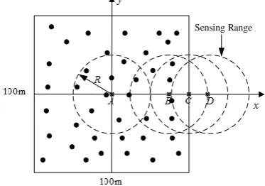
Usually the sensing range is controllable by improvement of threshold value, for the best utilization of sensor nodes with better SNR. However the sensing range of the sensor node directly affects the number of nodes that can detect the target. Fig.4 shows the detection circular area of each nodes. When the detection range of the sensor node is too small, the number of sensor nodes that can detect the target sound source in positions C and D may be less than four, and the positioning cannot be performed. In addition, for the target sound sources at positions A and B, if the sensor node detection range is too small, the number of sensor nodes that can detect the target sound source may also be less than 4, resulting in the inability to perform positioning. Assuming acoustic attenuation =2, White Gauss Noise square variance 2
0.01
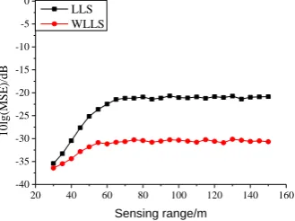
, sensing range R vary from 30m to 150m. Influence of Sensor node’s sensing range on localization accuracy is shown in Fig.5.
With the increase of sensor node detection range, the target positioning error becomes larger. Therefore, in practical applications, under the premise that the source can be located, the sensing range of the node should be reduced as much as possible by increasing the receiving threshold. As shown in Fig.5, localization accuracy keeps steady when node’s sensing range is larger than 60m at point A.
20 40 60 80 100 120 140 160
-40 -35 -30 -25 -20 -15 -10 -5 0
10
lg
(MS
E)/d
B
Sensing range/m
LLS WLLS
0.0 0.5 1.0 1.5 2.0
-35 -30 -25 -20 -15 -10 -5 0 5 10
10
lg
(MS
E)/d
B
[image:4.595.279.483.310.435.2] [image:4.595.107.272.312.435.2]Self-localizaition accuracy/m LLS WLLS
Figure 5. Influence of Sensor node’s sensing range. Figure 6. Influence of node’s location accuracy.
Influence of Nodes’ Location on Localization Accuracy
Location information of random distributed nodes in WASN is available through GPS localization or self-localization algorithm, but errors will happen whatever approach adopted. Requirement for senor location information is strict in target localization algorithm, so the influence of nodes’ location on the accuracy of algorithm deserves a research. In this study, acoustic attenuation coefficient =2, Square Variance of Gauss White Noise 2 0.01, also each nodes is able to detect the target. Fig.6 shows localization error of the target goes up with the increase of node’s location error. WLLS has more accuracy localization ability than LLS if node’s location error is small. While in contrast, LLS has better performance if location error is larger. Location error accumulated one time in LLS, but it is doubled in WLLS since weight in the algorithm calculated by the nodes location.
Influence of Attenuation on Localization Accuracy
calculated attenuation value. While if the actual attenuation value is smaller than two or larger than three, then the localized error will get larger, as shown in Fig.7.
1 2 3 4 5
-40 -30 -20 -10 0 10 20 30
in actual environment
10
lg
(MS
E)/d
B
LLS WLLS
1 2 3 4 5
-10 0 10 20
in actual environment
10
lg
(MS
E)/d
B
LLS WLLS
1 2 3 4 5
0 10 20
in actual environment
10
lg
(MS
E)/d
B
LLS WLLS
[image:5.595.63.536.93.235.2](a) =2 (b) =3 (c) =4
Figure 7. Localization accuracy with different attenuation coefficient.
Experimental Validation
Sensor nodes’ location information is required for target localization in WLLS. In order to specifically verify the validity of the positioning algorithm, the nodes are deployed in a preset manner, as shown in Fig.8. Coordinate of sensor 1 in this figure was set (0, 0) , as the original point, coordinate for the others three sensor are(10,0), (10,10),(5,10). Four points cannot be located on one circle, or there will be no solutions. This is not a problem in practical applications because the number of sensor nodes that can detect the target is large, so the algorithm always has solutions. Gate node places far enough to the sensors. Sound source played by recorder, places at coordinate A(5,5), B(10,5), C(12,5).
Node 1 Node 2
Node 3 Node 4
Gateway Node
[image:5.595.160.436.414.528.2]A B C
Figure 8. Nodes deployment for target localization by WLLS algorithm.
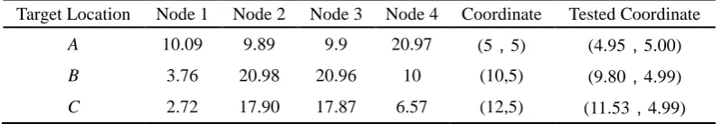
The energy value obtained by short-time energy processing after detecting the target noise will be converged to the gateway node. And the gateway node estimates the target position according to the WLLS. The sound energy value received by each node and the positioning result can be transmitted to the computer through the gateway node serial port. The experimental results are shown in Table 1.
Table 1. Experimental results.
Target Location Node 1 Node 2 Node 3 Node 4 Coordinate Tested Coordinate
A 10.09 9.89 9.9 20.97 (5,5) (4.95,5.00)
B 3.76 20.98 20.96 10 (10,5) (9.80,4.99)
C 2.72 17.90 17.87 6.57 (12,5) (11.53,4.99)
[image:5.595.99.499.631.700.2]Conclusion
Target localization algorithm based on weighted least squares is widely used in energy-constrained wireless acoustic sensor networks. This paper analyzes the main error sources that affect the positioning accuracy. The closer the target is to the center of the WASN, the more accurate the target position estimate. When the sound attenuation coefficient is 2 to 3 in the actual environment, the obtained positioning error is small. The smaller the node's sensing range is, the higher the target positioning accuracy is. However, when the radius of the sensing range of the node is 30 m or less, the number of nodes that can sense the target noise is too small to be positioned. When the position error of the node changes from 0 to 2 m, the position error of the WLLS varies from -30 dB to 6 dB. In the target location experiment using the pre-set node position, the WLLS target location algorithm can estimate the target’s position accurately, and the positioning error in both x and y directions is controlled within 0.5m.
References
[1] X. Zheng, R. Liyang. A Self-organizing Bearings-only Target Tracking Algorithm in Wireless Sensor Network [J]. Chinese Journal of Aeronautics, 22(6): 627-636, 2009.
[2] R. Liyang, X. Zhen. A Fast Global Node Selection Algorithm for Bearings-only Target Localization [J]. Chinese Journal of Aeronautics, 21(1): 61-70, 2008.
[3] R. W. Ouyang, A.K. Wong, C. Lea, Received Signal Strength-Based Wireless Localization via Semidefinite Programming: Noncooperative and Cooperative Schemes [J]. IEEE Transaction on Vehicular Technology, 59(3): 1307-1318, 2010.
[4] C. Meng, Z. Ding, S. Dasgupta, A semidefinite programming approach to source localization in wireless sensor networks, IEEE Signal Process Letter., vol. 15, pp. 253-256, 2008.
[5] W. Meng, W. Xiao, L. Xie, An Efficient EM Algorithm for Energy-Based Multisource Localization in Wireless Sensor Networks[J]. IEEE Transactions on Instrumentation and Measurement, 60(3): 1017-1027, 2011.
[6] P. Tarrio, A. M. Bernardos, J.A. Besada, A New Positioning Technique for RSS-Based Localization Based on a Weighted Least Squares Estimato. International Symposium on Wireless Communication System, 663-637, 2008.
[7] H. C. So, L. Lin, Linear Least Squares Approach for Accurate Received Signal Strength Based Source Localization [J]. IEEE Transactions on Signal Processing, 2011, 59(8): 4035-4040.
[8] J. Yuan, W. Ai, H. Deng, Exact Solution of an Approximate Weighted Least Squares Estimate of Energy Based Source Localization in Sensor Networks[J]. IEEE Transactions on Vehicular Technology, 64(10): 4645-4654, 2015.