2018 2nd International Conference on Modeling, Simulation and Optimization Technologies and Applications (MSOTA 2018) ISBN: 978-1-60595-594-0
Design and Analysis of a New Type of Tracking Differentiator
Xing-ge LI
1, Gang LI
2,*and Xu-chao KANG
11Graduate College, Air Force Engineering University, Xi’an 710051, China
2Air and Missile Defense College, Air Force Engineering University, Xi’an 710051, China
*Corresponding author
Keywords: Tracking differentiator, Differential signals, Stable, Nonlinear characteristics, Parameter setting rule.
Abstract. In this paper, a new tracking differentiator is proposed based on the inverse hyperbolic
tangent function. Due to the complexity of the tracking differentiator and the inaccuracy of tracking accuracy, accurate differential signals cannot be obtained. It is globally asymptotically stable, and its singularities are stable nodes by proper selection of parameters. The inverse hyperbolic tangent acceleration function has strong nonlinear characteristics, simple structure, less parameters and convenient adjustment. The simulation results show that NTTD is not only simple in structure form and relatively less in design parameters, but also has some advantages in tracking precision, response time and filtering ability.
Introduction
The accurate extraction of differential signals is very important in the design of control systems [1]. Especially when the system has external interference, the traditional lowpass filter is very difficult to play. In recent years, with the rapid rise of robots[2,3], hypersonic vehicles [4,5]and other fields, the extraction of accurate differential signals from interfered signals has become a hot spot of research.
The tracking differentiator was first proposed by Han Jingqing[6-8]. In his own article, he proposed three kinds of tracking differentiator, but the effect of tracking differential is not very good, and there is no good method for the problem of high order signal extraction. In recent years, many scholars have put forward a new tracking differentiator[9-12]. The Israeli scholar, Levent, proposed a high order sliding mode differentiator for the problem of high order differentiator[13]. However, the differentiator is very sensitive to noise and it is difficult to select the parameters. Therefore, it is necessary to design a tracking differentiator which is easy to select parameters and has the ability of noise suppression.
Based on the above considerations, this paper proposes a new tracking differentiator based on the inverse hyperbolic tangent function, and extends the tracking differentiator to higher order signals.
Design of Tracking Differentiator
In the conventional state, two conditions need to be satisfied to achieve stable tracking of the interfered differential signals. First, it has a smooth and stable property under the linear region near zero point, and then in the nonlinear region far away from zero, it needs to have strong nonlinear characteristics to ensure the stable tracking of the tracking differentiator. For this reason, the inverse hyperbolic tangent function is chosen as the acceleration function of differentiator.
Design of Two Order Tracking Function. Theorem 1 For the following system
1 2
2 1artanh( )1 2artanh( )2
z z
z a z a z
In the equation, a1>0 and a2>0 are the design parameters, z1R and z2 R are state variables. Then the system (1) is globally asymptotically stable at the origin (0,0).That is lim 1 0
tz and tlimz20.
Proof Select the Lyapunov function as
1 2
1 2 1 2
0
1 ( , ) artanh( )
2 z
V z z
a d z (2)Because a1>0, and when z1 >0, a1artanh(ξ)>0; when z1<0, a1artanh(ξ)<0, according to the integral mean value theorem, you can get.
1
1 1 1
0 artanh( ) = artanh( )
z
a d a z
(3) Which is, 0<ζ<z1,then 11
0 artanh( ) 0
z
a d
. And because, when z2≠0, 22 2 0
z , so
1 2
( , ) 0
V z z (4) And there is,
1 2 1 1 1 2 2 2 1 1 2 1 1 2 2 2 2 2
( , ) artanh( ) + z z artanh( ) + z [ artanh( ) artanh( )] artanh( )
V z z z a z z a z a z a z z a z (5)
In the same way, because of a2>0, there is, so you can get V z z( ,1 2)0. In the vicinity of the origin
(0, 0), only when z2=0, V z z( ,1 2) 0= . Therefore, according to the Lyapunov second theorem, the system
(1) is asymptotically stable at the origin (0, 0).
Design ofDifferentiator. Theorem 2 For the following system
1 2
2 2
2 1 1 2 2
( ) ( )
( ) artanh[ ( ) ( )] artanh[ ( ) ]
x t x t
x t a R x t u t a R x t R
(6)
Among them: u(t) is the input signal of the system; x1(t) is the system tracking signal; x2(t) is the differential signals of the system; R>0, a1>0, a2>0 are the adjust parameters of the system.
In order to prove that theorem 2 is correct, lemma 1 is first proposed.
Lemma 1 [7] For the following system
1 2
2 1 2
( ) ( )
( ) ( ( ), ( ))
y t y t
y t f y t y t
(7)
If any solution satisfies y t1
0,y t2
0(t ), then for any constant T>0 and any boundedintegrable function v(t)
1 2
2
2 1 2
( ) ( )
( ) ( ( ) ( ), ( ) )
x t x t
x t R f x t v t x t R
(8)
The solution of the system x1(t) satisfies
1 0
lim T ( ) ( ) 0
R
x t v t dt (9)The lemma theoretically clarifies the system in any time constant T, when the R tends to infinity, the system tracking signal x1(t) infinitely close to the input signal of the system v(t). Therefore, the system proposed in theorem 2 is the new tracking differentiator NTTD.
Phase Plane Analysis
For system (1), if we make 1
2
( ) 0
( ) 0
x t
x t
, we can get unique singularities (0,0).
The Jacoby matrix of the system (1) at the origin (0,0)
2 2
1 2
0 1
A
R a R a
(10) The x1 in system (6) is expanded by using Taylor's formula, you can get
1 2 ( 1 2)
x x x x, (11) The x2 in system (6) is expanded by using Taylor's formula, you can get
2 2
2 1 1 2 2 ( ,1 2)
x R a x R a x x x (12) Where φ andφ are higher order small quantities of Taylor expansion respectively, the linear system corresponding to system (6) is
1
2 2
2 1 1 2 2
2
( ) ( )
( )
x t t
x t R a x
x R a x
(13)
For linear approximation systems (13), we need to discuss the type of singularities separately. The eigenvalues of A are
2 2 1,2
2
R a
(14)
Where, 2 2
2 1
(a-4 )
R a
. When 2 2
2 1
( -4 ) 0
R a a , 2
2 4 1
a a is obtained, and the singularity (0, 0) is the stable node of the system. When x takes different values, the phase trajectories of the differentiator system always go parallel to the singularity (0, 0) in the same 2 directions. It can also be found that when the singularity is the stable node type, the system is directly convergent, and the oscillation of the tracking differential system in the over process is relatively small.
Parameter Setting Rule
According to the phase plane, the system (6) contains 3 parameters:R, a1, a2, Among them, R is related to tracking effect, which will increase the tracking rapidity, but increase the differential signal high frequency noise. The effect of a1 is related to the tracking effect, and its effect is similar to that of R; The a2 is related to the differential effect, which is beneficial to the suppression of differential noise, but the general assembly makes the tracking slow. Generally, the R can generally be roughly selected to adjust the tracking effect. Finally, the integrated effect of tracking and differential is adjusted by the micro tuning of a1 and a2.
Simulation Verification
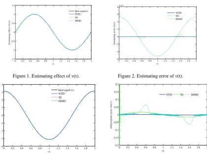
In order to verify the estimation results of NTTD, NTTD is compared with the following new TD[16] and HSMD[13].
The four step Runge-Kutta method is used to solve the simulation, and the simulation step is 0.001s. The simulation is carried out in the following two cases.
0 0.2 0.4 0.6 0.8 1 1.2 1.4 1.6 1.8 2 -1.5 -1 -0.5 0 0.5 1 1.5 E s ti m a ti n g e ff e c t o f υ ( t ) t/s
Ideal signalυ(t) NTTD TD HSMD
0 0.2 0.4 0.6 0.8 1 1.2 1.4 1.6 1.8 2 -6 -4 -2 0 2 4 6 8x 10
[image:4.595.98.520.66.397.2]-3 E st im a ti n g e rr o r o f υ( t) t/s NTTD TD HSMD
Figure 1. Estimating effect of ν(t). Figure 2. Estimating error of ν(t).
0 0.2 0.4 0.6 0.8 1 1.2 1.4 1.6 1.8 2 -4 -3 -2 -1 0 1 2 3 4 D if fe re n ti a l e ff e c t o f υ( t) t/s
Ideal signal υ(t) NTTD TD HSMD
0 0.2 0.4 0.6 0.8 1 1.2 1.4 1.6 1.8 2 -0.2 -0.15 -0.1 -0.05 0 0.05 0.1 0.15 0.2 d if fe re n ti a l e rr o r o f υ( t) t/s
NTTD TD HSMD
Figure 3. Differential effect of ν(t). Figure 4. Differential error of ν(t).
The estimation results of three differentiators and their differential values are shown in figure 1~figure 4. Figure 2 and Figure 4 show that in the three differentiators, the estimated error of NTTD pairs is the smallest and the accuracy is the highest. From Figure 4, we can see that NTTD has a more serious peak phenomenon, and HSMD has a serious buffeting phenomenon near 0. Therefore, when the noise is not considered, the NTTD proposed in this paper has certain advantages over TD and HSMD.
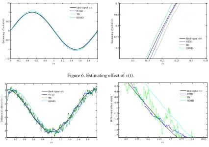
Simulation two: the input signal is taken and assumed to be polluted by random noise (see Figure 5). The design parameters of NTTD are: R=70, a1=90, a2=1.
[image:4.595.203.406.528.655.2]0 0.2 0.4 0.6 0.8 1 1.2 1.4 1.6 1.8 2 -1.5 -1 -0.5 0 0.5 1 1.5 υ ( t ) t/s Input signals received by noise pollution υ(t)
Figure 5. Input signal contaminated by noise.
0 0.2 0.4 0.6 0.8 1 1.2 1.4 1.6 1.8 2 -1.5 -1 -0.5 0 0.5 1 1.5 E st im a ti n g e ff e c t o f υ ( t ) t/s
Ideal signal υ(t) NTTD TD HSMD
0.1 0.15 0.2 0.25 0.3 0.35 0.5 0.55 0.6 0.65 0.7 E st im a ti n g e ff e c t o f υ( t) t/s
[image:5.595.92.519.69.370.2]Ideal signal υ(t) NTTD TD HSMD
Figure 6. Estimating effect of ν(t).
0 0.2 0.4 0.6 0.8 1 1.2 1.4 1.6 1.8 2 -4 -3 -2 -1 0 1 2 3 4 D if fe re n ti a l e ff e c t o f υ( t) t/s Ideal signal υ(t) NTTD TD HSMD
0.5 0.55 0.6 0.65 0.7 0.75 0.8 0.85 -2 -1.8 -1.6 -1.4 -1.2 -1 -0.8 -0.6 -0.4 -0.2 D if fe re n ti a l e ff e c t o f υ( t) t/s
Ideal signal υ(t) NTTD TD HSMD
Figure 7. Differential effect of ν(t).
Summary
In this paper, a new tracking differentiator is designed based on the inverse hyperbolic tangent function. It is globally asymptotically stable, and its singularities are stable nodes by proper selection of parameters. The inverse hyperbolic tangent acceleration function has strong nonlinear characteristics, simple structure, less parameters and convenient adjustment. The simulation results show that NTTD is not only simple in structure form and relatively less in design parameters, but also has some advantages in tracking precision, response time and filtering ability.
Acknowledgement
This research was financially supported by the National Science Foundation of China (No. 61703424), Aeronautical Science Foundation of China (No. 20175896023).
References
[1] X.W. Bu, X.Y. Wu, Y.X. Chen, R.Y. Bai, Design of a class of new nonlinear disturbance observers based on tracking differentiators for uncertain dynamic systems, Int. J. Control. Autom. Syst. 13 (2015) 595–602. doi:10.1007/s12555-014-0173-6.
[2] X.J. Wei, Z.J. Wu, H.R. Karimi, Disturbance observer-based disturbance attenuation control for a class of stochastic systems, Automatica. 63 (2016) 21–25. doi:10.1016/j.automatica.2015.10.019.
[3] R. Cui, L. Chen, C. Yang, M. Chen, Extended State Observer-Based Integral Sliding Mode Control for an Underwater Robot With Unknown Disturbances and Uncertain Nonlinearities, IEEE Trans. Ind. Electron. 64 (2017) 6785–6795. doi:10.1109/TIE.2017.2694410.
[5] X. Shao, H. Wang, Back-stepping robust trajectory linearization control for hypersonic reentry vehicle via novel tracking differentiator, J. Franklin Inst. 353 (2016) 1957–1984.
[6] H. Jinqing, Y. Lulin, The Discrete Form of Tracking-Differentiator, J. Syst. Sci. Math. Sci. 19 (1999) 268–273.
[7] J. Han, A New Type of Controller: NLPID, Control Decis. (1994).
[8] J. Han, L. Yuan, The discrete form of tracking-differentiator, J. Syst. Math. 19 (1999).
[9] H. Feng, S. Li, A tracking differentiator based on Taylor expansion, Appl. Math. Lett. 26 (2013) 735–740. doi:10.1016/j.aml.2013.02.003.
[10] L. Zhang, Z. Zhang, L. Huang, Hybrid non-linear differentiator design for a permanent-electro magnetic suspension maglev system, IET Signal Process. 6 (2012) 559. doi:10.1049/iet-spr.2011.0264.
[11] A. Mohammadi, M. Tavakoli, H.J. Marquez, F. Hashemzadeh, Nonlinear disturbance observer design for robotic manipulators, Control Eng. Pract. 21 (2013) 253–267. doi:10.1016/j.conengprac.2012.10.008.
[12] T. Zhou, Extended state observer based on inverse hyperbolic sine function, Control Decis. (2015).
[13] A. Leventa, Robust exact differentiation via sliding mode technique*, Automatica. 34 (1998) 379–384.
[14] X.M. Dong, P. Zhang, Design and phase plane analysis of an arctangent-based tracking differentiator, Control Theory Appl. (2010).
[15] Y.Q. Liu, J.Y. Guo, Design and Phase Plane Analysis of a Hyperbolic Tangent Tracking Differentiator, Electr. Power Sci. Eng. (2017) 74–78.