A Novel Real Time Algorithm for Remote Sensing Lossless Data Compression based on Enhanced DPCM

A Novel Real Time Algorithm for Remote Sensing

Lossless Data Compression based on Enhanced DPCM

P. Ghamisi

Research Scholar Geodesy and Geomatics

Engineering Faculty, K.N.Toosi University of

Technology, No. 1346, Vali_Asr St.,

Tehran, Iran

A. Mohammadzadeh

Assistant Professor Geodesy and Geomatics

Engineering Faculty, K.N.Toosi University of

Technology, No. 1346, Vali_Asr St.,

Tehran, Iran

M. R. Sahebi

Assistant Professor Geodesy and Geomatics Engineering Faculty, K.N.Toosi University of

Technology, No. 1346, Vali_Asr St.,

Tehran, Iran

F. Sepehrband

PHD Student, CSE Department. University of New South Wales, Kensington,

Sydney, NSW 2032

J. Choupan

PHD Student, CSE Department. University of New South Wales, Kensington,

Sydney, NSW 2032

ABSTRACT

In this paper, simplicity of prediction models for image transformation is used to introduce a low complex and efficient lossless compression method for LiDAR rasterized data and RS grayscale images based on improving the energy compaction ability of prediction models. Further, proposed method is applied on some RS images and LiDAR test cases, and the results are evaluated and compared with other compression methods such as lossless JPEG and lossless version of JPEG2000. Results indicate that the proposed lossless compression method causes the high speed transmission system because of good compression ratio and simplicity and suggest to use in real time processing.

Keywords

Remote Sensing (RS), Lossless Compression, LiDAR Technology, Enhanced DPCM Transform.

1. INTRODUCTION

Light Detection And Ranging (LiDAR) can be used for providing elevation data that is so accurate, timely, and increasingly capable in inhospitable terrain [2] and is widely used in a lot of applications such as the investigation of atmospheric parameters, earth management, bare earth digital terrain models and so on.

In profiling and transmission of RS data, compression can be useful a lot. On the other hand, due to the important information that RS data contains, lossless compression is preferred. In addition, in real time applications, simple algorithm accelerates execution process time. Therefore, a fast and efficient compression algorithm can be very useful for RS data.

Lossless compression generally consists of two major parts, transformation and entropy encoding [3], [4]. There are a lot of methods available for lossless compression, which contain these

more supplementary steps. Joint Photographic Expert Group (JPEG) standards are widely used for image compression [5]. Few of these methods are efficient in compression but have high computational complexity and few are reverse. For example, JPEG2000 is powerful in compression but has high computational complexity.

In this paper, a low complex method for lossless compression of RS data is introduced based on enhanced DPCM transformation (EDT) and optimized Huffman encoder. The EDT improves the energy compaction ability of DPCM. The proposed method is efficient in compression ability and fast in implementation. Then, the adaptive scheme is introduced. Finally, our proposed method is applied on few RS grayscale images and LiDAR rasterized data test cases and results are evaluated.

This paper is organized as follow. Section 2 is devoted to background. Then, a brief introduction about LiDAR technology and images is brought in Section 3. Further, in Section 4, the proposed method is briefly introduced. Section 5 is devoted to the experimental results and comparison of the new method with previous methods. Finally, our conclusion remarks and future works are included in Section 6.

2. BACKGROUND

As mentioned in previous Section, JPEG standards are well-known compression methods which are widely used for image compression. Lossless JPEG, JPEG-LS and lossless version of JPEG2000 are lossless methods of JPEG standards that are going to be compared with the proposed method.

2.1 Lossless JPEG

neighboring pixel by a specific equation and calculating the error of prediction. The neighboring position and different predictor equations are shown in Fig. 1 [6].

Fig. 1. Neighboring Pixels in DPCM and Prediction Equations (Sepehrband 2011)

Better prediction causes the predicted pixel to be closer to the original pixel value, and, therefore, results in less prediction error value.

2.2 JPEG-LS

JPEG-LS standard of coding still images provides lossless and near-lossless compression. The baseline system or the lossless scheme is achieved by adaptive prediction, context modeling, and Golomb coding [7].

2.3 JPEG2000

JPEG2000 is based on the discrete wavelet transform (DWT), scalar quantization, context modeling, arithmetic coding, and post-compression rate allocation [7]. JPEG2000 works well and gives a good compression ratio especially for high-detail images, because it analyzes the details and the approximation in the transformation step and decorrelates them. However, JPEG2000 has high computational complexity.

3. LIDAR

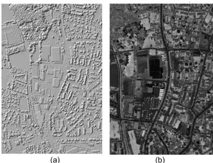
LiDAR technology is used to obtain elevation data with sending eye-safe near infrared laser light in the region of 1040 to 1060 nm and receive these pulses after encountered them to objects from the earth and evaluate the range of pulse traveling. A laser pulse moves with speed of light (3×108ms-1) therefore, the travel time of laser pulse from the transmitter to the target and back to the receiver can be measured accurately [8]. For converting these data to images, Inverse Distance Weighting (IDW) or Triangular Irregular Networks (TIN) applied to return data and portray them in shaded-relief forms for data validation and looking for anomalies and errors in the data [8]. Fig. 2. (a) indicates an example of these kinds of images that mentioned above.

Most LiDAR systems provide an intensity file in addition to the multiple return data [8]. The LiDAR intensity images are similar to panchromatic images and contain a wealth of details and information regarding to a lot of applications in remote sensing field. Fig. 2. b shows an instance of intensity images.

Fig. 2. Example of rasterized data. a)First Return, b)First Intensity

As can be seen from Fig. 2, LiDAR images have high neighboring correlation. Therefore, prediction models would be efficient for LiDAR rasterized data transformation. Because, possibility of correct prediction in the highly correlated images is more than other images and as a result, transformed image energy will be more compact. Therefore, transformed image will have less entropy value. Entropy or required bit per pixel shows the possibility of compression and is calculated as follow [9]:

(1)

where r is the intensity value, L is the number of intensity values used to present the image, and p(r) is the probability of intensities. For an image with a depth of 8 bits, L would be equal to 256 and r would be in the range of 0-255. The histogram of the given image can be used to calculate the intensities’ probabilities [9]. An image with less entropy value indicates that more compression is possible. Transformation increases energy compaction and, as a result, the probability of each intensity or source symbols increase leads to less redundancy and less entropy. Compression ratio can be obtained by dividing the size of original image by the size of the compressed bit-stream. Computational complexity is another factor that determines the efficiency of a method. It can be obtained by counting the number of CPU cycles or hardware gates and etc. These are dependent on target application (Ebrahimi 2000).

4. PROPOSED METHOD

Image(I) divided by n Input Image

X(i,j) is predicted Pick neighbors of X which are A,B,C and D

All pixels predicted No

Rescaling of predicted image

Yes

Save remainder

+

Predicted image is created now (P)

Store remainder Store first row

and column

Creating Huffman dictionary with only

even values

Huffman encoding Store coded

image

Store Huffman dictionary

+

Entropy encoding Enhanced

DPCM Transformation Calculating

prediction error (T)

Store compress bit-stream

Concatenation

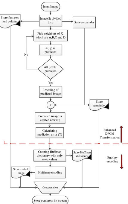
Fig. 3. Flowchart of Proposed Compression Method

4.1 Transformation (EDT)

EDT is based on predictive models. However, more energy compaction is obtained by improving the prediction ability. Energy compaction and low complexity are few important attributes of any good transformation (Sepehrband 2010). In hardware implementation point of view, the transformation method is obtained by adding only two shift register to previous DPCM. Therefore, complexity of EDT stays low. Our new transform method engine is illustrated in the block diagram form in Fig. 4. Division is first applied on the input image. Then, quotients of division are being predicted by one of the prediction equations of Fig. 1. Also, (2) can be use as the equation of the prediction step. Further, predicted matrix is re-scaled in the multiplication step. Furthermore, by adding the predicted matrix with the remainders of the division step, predicted image is produced. the subtraction of the predicted image from the original image gives the prediction error the matrix which is the transformed image [10] [1].

X = (2)

When intensities of an image are in the range of [0, 2k- 1], the image is of k-bit depth. Typical grayscale images are of 8 to 16

R, G and B each of which has the same depth to grayscale. In this paper, grayscale images with an 8-bit depth are focused on. As shown in Fig. 4, the input image is divided by n and the rounded quotient and the remainder of the division are kept in Quotient and Remainder, respectively. Divisor is chosen in a fashion that the sum of the quotient depth and the remainder depth is equal to the input image depth. Therefore, in an 8-bit depth image, divisor is a power of two and smaller than the biggest possible intensity value.

= (3)

For a specific n of (3), quotient and remainder are:

(4)

(5)

For input image I(i,j), intensities are in the following interval.

(6)

Therefore, from (4) and (5) for q(i,j) and r(i,j) we have:

,

,

,

(8)

(9)

Fig. 4. Block Diagram of New Transformation Method

Assume that a linear prediction model such as Prediction Number Five of Fig. 1 is being used, (X = B). Then, the probability of the correct prediction is the probability of that intensity value shown in (9). Rr is the number of repetition of

intensity r in an M × N image and Pr is the probability of r.

Therefore, in this case Pr will be the probability of the correct

prediction.

(9)

We have q(i,j) from (4), which is obtained by dividing each pixel of the input image by n. Hence, the probability of the correct prediction for q(i,j) is shown in (10). Rq is the number of repetition of the new intensity values q in the divided image.

(10)

- 1)/n

When one number is considered instead of a series of values in an interval, the total number of repetitions would increase. From (10), the new value of repetition Rq and then Pq are:

(11) 1≤ d ≤n

(12)

From (12), it can be easily deduced that the probability of the correct prediction would increase. In other words, it is obvious that the probability of the correct prediction in a smaller interval is higher than a bigger interval which leads to better prediction. The objective of our method is to estimate the prediction error, so it would be necessary to have a predicted image. Next, the predicted matrix is re-scaled by multiplying the predicted matrix by n and then, adding it to the remainder. Hence, the predicted image is calculated as:

(13)

In which qp(i; j) is the output of the prediction step it can be called the predicted matrix. Then, the prediction error which is the output of the transformation T(i,j) will be obtained by:

(14)

The transformed image by this method has less intensity distribution compared to DPCM. Therefore, more energy compaction will take place. This happens because the transformed image values have less variety than the output of DPCM. Actually, as it is shown by mathematical proof, variations of the transformed image values by this method is n times smaller. Similar to (13), I(I, j) can be calculated as:

(15)

r is equal in both (13) and (15). Hence, we can say:

(16)

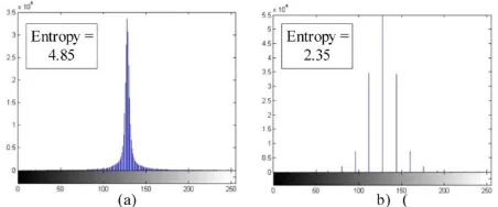
Fig. 5. Histogram of: a) Lossless JPEG transformation, b) Transformed image by new method with n = 32 of Barbara

image

From (14) and (16), we have (17) for transformed image.

(17)

As qp and q are in the range of [0, 2k-m - 1]:

– (18)

So all possible prediction error values Tv(i; j) for our transformation is calculated as:

V = 0, 1, . . . , 2k-m – 1 (19) According to (19), the variety of outputs for the new method is n times smaller than DPCM. So energy compaction is n times better, which is a good attribute. All outputs of the method are coefficients of n. The new method is applied on 512×512 Barbara image with an 8-bit depth by picking n equal to 32. Further, the histogram of lossless JPEG transformation output is compared with the histogram of the new method output in Fig. 5. From (19), the variety of prediction error values will be equal to ( Tv(I, j) = 32 × V ).

Where V is in the range of [0, 7]. Hence, there will be only 8 different possible values for the prediction error, which are [0, 32, 64, . . . , 224]. On the other hand, DPCM outputs have variety in the range of 0 to 255. As can be seen from Fig. 5, the new method causes less variety in the output and as a result more energy compaction and more redundancy reduction would be achieved. Hence, intensity distribution becomes n time fewer. Then, generally for V:

V = 2k / n = (20)

The entropy value decreased by enhancing the energy compaction and causes more compression. Assume an image with equal probability distribution for all intensities. Entropy can be calculated by (1) (Gonzales 2008). Then, for entropy of such image, we will have:

(21)

(22)

Ln is the number of intensities for the divided image. From (21)

and (22) for an image transformed by the new method:

E = - log2 (1/Ln) = - log2(n/L)

=k-m (23)

It means that the required bit per pixel or entropy value of the transformed image decreases and as a result, more compression would be achieved.

Lossless compression of RS data is our main purpose for introducing this method. Thus, n = 2 must be picked to prevent loss of information. Therefore, the only possible values for the remainder would be 0 or 1 and there would be no loss of critical information in the reconstruction phase. In images reconstruction phase, one failure in intensity value estimation (e.g. reconstructing 201 besides 200) cause about 0.39 percent of intensity change. This change could be disregarded. Another way to ensure that the method is completely lossless is to save or send remainders with the transformed image that is 1=8 of the main image. In this paper for achieving the completely lossless compression, the reminders are saved and used in the reconstruction phase. Lossy compression is achieved by applying bigger n for the division step. If we pick a very big n like 64, we may lose lots of information and the predicted image do not have an acceptable quality and as a result the reconstructed image will not have a good quality.

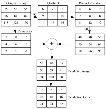
As an instance, the whole numerical process for the image of the last example is discussed in the following. A 3 × 3 part of Barbara image is incised and all the steps of the new method are shown in Fig. 6. n is equal to 8 for this example and prediction number one (X = (B +D)/2) is used. As can be seen in Fig. 6, all the values of prediction error are factors of 8. So all the energy will be compact into 32 different values which are:

Fig. 6. Numeric Example of the New Transformation

Tv(I, j) = 8 × V

V = 0, 1, . . . , 25 – 1 (= 31) (24)

It is almost certain from the numerical example that keeping the remainder helps a lot with this energy compaction because it makes the answers to be a factor of n. Also it should be noted that a good predictor gives better results.

4.2 Entropy Encoding

Huffman encoding is selected as the entropy encoder for the proposed lossless compression method. Huffman codes the image intensities due to their probability and forms them as a bit-stream. Therefore, Huffman dictionary, which includes intensity codes, needs to be saved as an overhead too. After calculating the prediction error, all the values are in the range of -2k + 1 and 2k - 1. For example, for a grayscale image with an 8-bit depth the interval is between -255 to 255. Therefore, Huffman needs a dictionary which covers this interval. To have an efficient encoder, it is decided to change the negative values of the transformed image to positive. This occurs in multiplying of the input image and the predicted image, as it is mentioned in (18). Absolute values are saved in subtraction process. As a result, the dictionary becomes smaller and needs to code only the symbols between 0 and 256. However, the signs need to be known for the reconstruction phase. To solve this problem, an extra overhead is added to the compressed image which includes the sign of each code in one bit. This overhead is 1/8 of the input image.

4.3 Reconstruction

The reconstruction phase consists of Huffman decoding and inverse transform of our transformation method. The inverse of the transformation is obtained by calculating the main values from the inverse of prediction equation. To achieve this goal and to have a complete reconstruction, the first row and the first column of the main image need to be saved and then, reconstruct each pixel from neighbors. Inverse transformation for pixel X of Fig. 1 is calculated as follow:

(25)

visually lossless compression, the remainder overhead can be ignored and more compression ratio would be achieved. For near-lossless or visually lossless transformation n is equal to 4. It causes at most 1.56 percent intensity changes in reconstruction of transformed image. Lossy compression is achieved by applying a bigger n for the division step. If a very big n such as 64 is picked, lots of information may be lost and the predicted image does not have an acceptable quality and as a result, reconstructed image will not have a good quality respectively. Therefore, it depends on the importance of the required quality for picking a divisor. For critical images with a lot of details, this study suggests using the lossless scheme for important parts and near lossless for other parts.

5. EXPERIMENTAL RESULT

5.1 Remote Sensing grayscale Images

In this section, the proposed method is tested on some RS grayscale images. To achieve this aim, 10 RS grayscale images were picked and the proposed method is applied on them. RS test images include information about earth in the digital form which were captured by satellites in different spatial resolutions. In these images, each pixel has a grayscale value from 0 (Black) to 255 (White). Any of these pixels represents a specific region of earth. Our test cases are 8-bit depth images in different sizes from 300 × 450 to 1893 × 1825. Fig. 7 illustrates an example of one of our RS test images from the town of Dessau on the Elbe River in Saxony-Anhalt, Germany which was captured by Landsat thematic mapper (TM) sensor with a 30 meters of spatial resolution. These images were selected from ENVI and eCognition softwares. Our main focus was on lossless compression of RS images. To provide lossless compression, we picked n=2 as the divisor. Also, we applied this method on 10 grayscale satellite images. Lossless JPEG results are obtained using MATLAB and JPEG2000 results are calculated using ENVI© software version 4.4.

Fig. 7. the town of Dessau on the Elbe River in Saxony-Anhalt, Germany, Landsat TM

Table I illustrates our investigation on RS test images. For various kinds of test images, results indicate that the proposed compression method improved lossless JPEG compression ratio about 7 percent and JPEG2000 more than 3.5 percent. On the other hand, the new method improved the average compression ratio of Lossless JPEG about 0.3 and JPEG2000 about 0.28. In proposed Method, different equation in Fig. 1 cause different compression ratio. Better prediction which caused less error in prediction error estimation. Thus more energy compaction and more entropy reduction will be obtained. These factors lead us to obtain more compression ratio. According to detail analysis of JPEG2000’s transformation scheme, JPEG2000 is efficient in high detailed images. However, the proposed method generally gives better result in comparison with JPEG2000.

Table 1 Average Compression Ratio Of Ten Different RS Grayscale Images,

Image Number

Lossless JPEG

JPEG2000 Proposed Method with EDT

1 1.31 1.41 1.46

2 1.38 1.38 1.73

3 1.31 1.25 1.76

4 1.24 1.29 1.46

5 1.19 1.20 1.34

6 1.48 1.47 1.90

7 1.34 1.42 1.57

8 1.49 1.38 1.95

9 1.23 1.23 1.57

10 1.32 1.40 1.60

Average 1.3273 1.3422 1.6326

5.2 LiDAR Rasterized Data

Table 2Compression Ratio of Different Standard Test Images of Lidar Rasterized Data (Ghamisi 2011) Image

Number

Lossles s JPEG

JPEG

2000

Proposed Method with

EDT

Proposed Method with

AEDT

1 1.234 1.275 1.426 1.64

2 1.3376 1.3374 1.7178 1.9681

3 2.4782 2.5604 2.9623 3.3986

4 1.3295 1.3282 1.7053 1.9513

5.3 Computational complexity

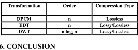
Table III illustrates the computational complexity of different transformation methods and the compression type which is used for comparison. The order of algorithm is O(n) in which n is the number of pixels or M × N. As can be seen in Table III, the complexities are compared. The comparison is based on the order of each transformation that may increase if a time consuming loop occur. Due to the fact that EDT and DPCM does not have any filter banking procedure or convolution, they less computational complexity than transformation of JPEG2000 (DWT). EDT has the same order as DPCM, because there is no more hierarchical loop is added to the old DPCM algorithm. According to the additional division and multiplication process in EDT, it has a slightly higher computational complexity than lossless JPEG. To avoid this problem and to have a less complex lossless scheme, shift with carry is used. So, the remainder of the dividing process is saved in carry. Then, in the re-scaling process, one left shift with carry would be used to add the remainder to the predicted matrix. Hence, the process of reconsidering the reminder would be omitted and the total computational complexity will decrease. Therefore, it can be concluded that, our proposed lossless transformation is achieved by adding only two shift registers to transformation of lossless JPEG and as a result, complexity stays low. It should be noted that choosing a less complex predictor such as X = B, can decrease the total computational complexity and accelerate the transformation process. For example, predictor X = (B +D)/2 needs a one bit shift register and an adder block, but X = B can be implemented by only one selector. Due to the high neighboring correlation of RS images, predictor X = B is an efficient one in the purpose of redundancy reduction too.

Table 3 Computational Complexity Of Different Transformations

Transformation Order Compression Type

DPCM n Lossless

EDT n Lossy/Lossless

DWT n log2 n Lossy/Lossless

6. CONCLUSION

In this paper, an efficient method for lossless compression of LiDAR rasterized data and RS grayscale images has been introduced in a way that, the proposed method is suitable for real time applications. As the hardware implementation accelerates the real time applications process, suitability satisfied by introducing a low complex and fast algorithm. However,

few previous methods such as lossless JPEG and JPEG2000 in both of RS grayscale images and LiDAR rasterized data. The compression ratio improvement helps transmission systems to work faster and helps the real time process. The proposed method is based on Enhanced DPCM Transformation (EDT) and optimized Huffman entropy encoder. The future studies would be on, hardware implementation, testing and evaluation.

7. REFERENCES

[1] Ghamisi, P. and Sepehrband. F, and Mohammadzadeh, A. and Mortazavi, M. and Choupan, J., 2011. “Fast and efficient algorithm for real time lossless compression of lidar rasterized data based on improving energy compaction,” in 6th IEEE GRSS and ISPRS Joint Workshop on Remote Sensing and Data Fusion over Urban Areas, Munich, Germany,

[2] McGlone, J. C., 2004. Manual of photogrammetry. Bethesda: ASPRS, vol. fifth.

[3] Foos, E. M. and Slone, R. and Erickson, B. and Flynn, M. and Clunie, D. and Hildebrand, L. and Kohm, K. and Young, S., 2000 . “Jpeg2000 compression of medical imagery,” in DICOM SPIE MI, vol. 3980, San Diego. [4] Calderbank, R. and Daubechies, I. and Sweldens, W. and

Yeo, B. L., Oct 1997, “Lossless image compression using integer to integer wavelet transforms,” in Proc. ICIP-97, IEEE International Conference on Image, vol. 1, Santa Barbara, Callifornia, pp. 596–599.

[5] Skodras, A. and Christopoulos, C. and Ebrahimi, T., sept 2001. “The jpeg2000 still image compression standard,” IEEE Signal Processing Magazine, pp. 36–58.

[6] Sepehrband, F. and Choupan, J. and Mortazavi, M., 2011 “Simple and effcient lossless and near-lossless transformation method for grayscale medical images,” in SPIE medical imaging, Florida, USA.

[7] Ebrahimi, T. and Cruz D. S. and Askelof, J. and Larsson, M. and Christopoulos, C., 2000. “Jpeg 2000 still image coding versus other standards,” in SPIE Int. Symposium, San Diego California USA, 30 Jul - 4, invited paper in Special Session on JPEG2000.

[8] Jensen, J. R, 2007. Remote sensing of environment: an earth recourse perspective. University of South Carolina, vol. second.

[9] Gonzales. R and Woods, R., 2008, Digital Image Processing, 3rd ed. New Jersey: Pearson Prentice Hall, Upper Saddle River,, pp. 525-626.

[10] Sepehrband, F. and Ghamisi, P. and Mortazavi, M. and Choupan, J., December 2010 “Simple and efficient remote sensing image transformation for lossless compression,” in ICSIP proc., Changsha, China.

[11] Starosolski, R., , 2007. “Simple fast and adaptive lossless image compression algorithm,” SOFTWARE-PRACTICE AND EXPERIENCE, Wiley InterScience, pp. 37–56. [12] Savakis, A. and Piorun, M. , Sept 2002, “Benchmarking