An Alternative of Poverty Line Measurement: a Case Study of Indonesia

Munich Personal RePEc Archive

An Alternative of Poverty Line

Measurement: a Case Study of Indonesia

Widodo, Tri

Economics Department, Faculty of Economic and Business,

Universitas Gadjah Mada, Indonesia

28 June 2001

Online at

https://mpra.ub.uni-muenchen.de/78323/

An Alternative of Poverty Line Measurement: a Case Study of Indonesia

By:

Tri Widodo

An Alternative of Poverty Line Measurement: a Case Study of Indonesia

Abstract

This paper discusses poverty lines in Indonesia. Firstly, the various poverty lines in Indonesia is discussed. The differences in methodologies and assumptions had created the central controversies in determining the poverty lines: kinds and quantities of goods. Secondly, an alternative poverty line measurement is the theoretically derived under Linear Expenditure

System (LES). This poverty line might overcome the controversies. Thirdly, the poverty line

measurement is then applied in case of Indonesia. This paper consludes that the economic crisis in 1997 had led to the increase of poverty lines in urban areas higher than in rural area.

Keyword: Poverty Line, Linear Expenditure System (LES), Seemingly Uncorrelated Regression (SUR).

JEL: D11, D60

I. Background

A simple question is sometime addressed: who is the poor? The answers to this

question are still debatable. There are some definitions of poor people. Defining poverty is a

matter of social convention (Pradhan 2000:2). An obviously and universally accepted

definition of poverty, unlike the presence of its real problem, is somehow hard to define.

There are a lot of definitions of poverty which can be used to different countries or regions

and at all times, independent of the social structure and level of development (Meier,

1995:26). Some would go into a pragmatic conclusion by looking at poverty as merely

contextual and can not be conceptualized since the notion of ‘being poor’ or ‘feeling poor’

can be very subjective (Widodo, 2002). However, for analytical and policy purposes, a

rigorous definition is required.

There were at least three definitions of poverty line in most highly publicized research.

(Badan Pusat Statistik, BPS). The second one was a measurement proposed by the

International Labor Organization (ILO) and the United Nations Development Program

(UNDP). The third measurement was published by the World Bank, SMERU – a

non-governmental organization funded by the World Bank – and a joint study by RAND Graduate

School and Demographic Institute, Faculty of Economics, University of Indonesia.

It can be argued that those immediate poverty measures might not be representing the

real condition, since they were not based on the appropriate data. But it is reasonable, since

the poverty alleviation policies were urgently needed, and it requires a quick estimation on

poverty. The lesson is that in the future, there is a need for a method for poverty measurement

that is justifiable, acceptable and applicable.

This paper aims to formulate an alternative measurements of poverty line which

theoretically acceptable. The standard maximization utility in microeconomics will be applied

to derive the alternative measurement of poverty line. And then, the alternative measurement

derived is simulated by using Indonesian data. The rest of this paper is organized as follows.

Part II presents literature study of poverty line. Part III exhibits the methodology applied in

this research. This part mainly presents the derivation of poverty line under Linear

Expenditure System (LES). Estimate and some simulations are presented in Part IV. Part V

exhibits some conclusions..

II. Literature Study

Poverty is not the same with inequality. Where as poverty is related with the absolute

standard of living of a part of society – the poor – inequality refers to relative living standard

inequality is possible with zero poverty (where no one is poor) as well as with maximum

poverty (where all are poor).

The perception of poverty has changed tremendously and evolved historically from

culture to culture. Criteria for determining poor and non-poor tend to express particular

national priorities and normative concepts of welfare and rights. It is common that as

countries become wealthier, their perception of the acceptable poverty line changes.

What is poverty? A simple definition of poverty is the inability to attain a minimal

standard of living (Meier 1995:26). Similarly, it is the inability of an individual or a family to

command sufficient resources to satisfy basic needs (Fields 1994:88). It delivers a commonly

shared idea of poverty as a state of deprivation. Despite giving a general idea, such definition

also provides more issues to explore. This opens the room for some possible approaches in

discussing poverty. Rein (1971) determines three approaches namely: (1) the biological

approach, (2) the inequality approach, and (3) the externality approach.

The biological approach defines the poor as those who earnings are not enough to

obtain the minimum necessities for maintaining physical efficiency. This approach was

derived from the famous work of Rowntree (1901). Having nutritional standards on deriving

the poverty line, malnutrition and starvation are clear symptom of the presence of poverty.

This approach is subject to some vagueness and limitations. Sen (1981) noted several

problems on implementing such approach. First, there are significant variations related to

physical features, climatic conditions and work habits. The survival ability may vary across

societies and over different period of time. Second, translating the minimum nutritional

requirement into minimum food requirement, which depends on the choice of (food)

non-food expenditure. A usual way to solve this problem is by assuming arbitrarily that a

family or individual will spend a certain proportion of their income for food consumption.

Subtracting this amount, we can calculate the non-food expenditure.

The second approach, inequality approach, covers a comparison of economic

positions. It is often argued that inequality and poverty are two separated things. Although

both concepts are associated to each other, basically they are not equivalent. However, both

concern the same idea that poverty is the state of deprivation. (Meier, 1995:25). This approach

focuses more on the nature and size of the difference between different groups in the society

instead of focusing on the (absolute) poverty line. Townsend (1974, 1979) argues that poverty

should be defined only in terms of relative deprivation. That is, not in how wealthy is an

individual, but in how less wealthy he or she is compared to the other members of the society.

Accordingly, the need for a ‘reference group’ is an important implication of applying

the concept in empirical analysis. The choice of it is in order to “define the style of living

which is generally shared or approved in each society” (Townsend 1974:36). The other

groups in society, which have less entitlement of resources, are compared to this reference

group. Although the approach can eliminate the static characteristics of the first one, however

it appears to be difficult to keep certain analysis to be value-free.

The third approach, the externality approach,is related with the “social consequences

of poverty for the rest of society rather than in terms of the need of the poor” (Ariffin 1992:2).

This view was originally introduced by Rein (1971). Presenting his argument he noted that the

concept of poverty “must be seen in the context of society as a whole”. He then quoted

Smolensky (1966) that poverty line should serve as an “index of the disutility to the

Poverty Line in Indonesia

There are various approaches had been used to derive the poverty line before the

official poverty line in Indonesia was published by the BPS in 1984. Some well-quoted

approaches are Sajogyo (1975), World Bank (1980), Booth (1981), Rao (1983) and a latter

work by Esmara (1986). The official poverty line method adopted by the BPS since 1984 is a

two-step method, combining the separate food and non-food poverty lines.

The first component, ‘food poverty line’ (FPL), is derived using the Food

-Energy-Intake (FEI) method. This method considers the basic human needs for food as energy

(calorie) fulfillment. A minimum calorie requirement is set up as 2,100 calories per day. The

food poverty line is then defined, as the minimum expenditure needed to purchase such level

of calories. For monthly per capita expenditure, the average price of calorie was computed by

dividing the monthly expenditure for food by per capita calorie intake (Sutanto et al. 1999:3).

The second component, Non-Food Allowance (NFA), in addition to the FPL is more

complex. The reason is that, unlike the presence of FEI assumption for FPL, there are no clear

base for assigning the non-food basic needs. Also in many cases in developing countries, the

price information availability for non-food commodities are difficult to get. Therefore the

non-food expenditure should be estimated.

The method used by the BPS was applying a certain mark-up to the FPL as the

estimation for NFA. The mark-up was based on several commodities, considered to be the

basic non-food goods. The combination of FPL and its mark-up is the final poverty line. This

method is, however, subject to the arbitrariness on choosing the goods. In 1993, the BPS

commodity bundle is based on the living standard of a ‘reference population’. The reference

population is a class of population whose income is just above the expected poverty line.

Although the reference population method is slightly better than just arbitrarily

determine the commodity bundle, the choice of the reference population itself is still based on

subjectivity. In addition, it also seems to have circularity problem since to derive the exact

poverty line, one has to have an ‘expected value’ of poverty line in his or her mind, in order to

choose the reference population.

The BPS defined two poverty line in the its first publication of poverty figures: first,

batas miskin(the ‘poverty line’ that is referred to as the ‘overall poverty line’, OPL); second,

batas sangat miskin (the ‘very poor line’, henceforth referred to as the ‘food poverty line,

FPL). The latter appeals the level of income needed to cover expenditure on the food

component of the expenditure basket reflected in OPL. Since 1984, the BPS has not reported

figures for ‘food poverty line’ (meaning food components of the overall poverty line).

There are some changes in calculating the poverty line therefore some problems arise.

The 1998 poverty line were derived using a much smaller sample survey (10,000 household)

than the usual Susenas1, whose sample size is aroud 65,000 households. It does not allow to

derive the poverty line by province. The 1998 poverty line derived by the BPS result in a ratio

of urban to rural overall poverty lines of 1.33 and of the urban to rural food poverty lines of

1.25 (Asra 1999:53). The food basket method used to develop the poverty lines allows for

different food patterns (i.e. consumption of different quantities of food items) in urban and

rural areas, where as the methodology applied until 1993 allowed for different calorie

consumption patterns. The reason for applying different sets of quantity weights for urban and

rural areas is to reflect the specific characteristics of each area, so that the poverty line is

‘location specific’ (Asra 1999:53) .

Table 1. The Criteria and Poverty Line

Research Criteria

Poverty Line

Urban Rural Urban+Rural

Esmara (1969/1970) a)

Consumption of rice per capita per year (kg) - - 125

Sayogya a)

1971

Expenditure level of rice equivalence per capita per year:

- Poor - Very poor - Poorest 480 360 270 320 240 180 - - - Ginneken a)

1969

Minimum of nutrition need per capita per day - Calorie

- Protein (gram)

- - - - 2,000 50 Anne Both a)

1969/1970

Minimum of nutrition need per capita per day - Calorie

- Protein (gram)

- - - - 2,000 40 Gupta a)

1973

Minimum of nutrition need per capita per year (Rp)

- - 24,000

Hasan a)

1975

Minimum income per capita per year (US $) 125 95 -

BPS b)

1984

1. Calorie per capita per day

2. Expenditure per capita per day (Rp)

- 13,731 - 7,746 2,100 - Sayogya b)

1984

Expenditure per capita per day (Rp) 8,240 6,585 -

World Bank b)

1984

Expenditure per capita per day (Rp) 6,719 4,479 -

International Poverty lines

1. Interim report 1976 b)

2. Ahluwalia 1975 c)

Income per capita per year: - value US $ 1970

- purchasing power parity US $ Level of income per capita per year (US $)

- - - - - - 75 200 50 75 Note:

a) Esmara, H., 1986. Perencanaan dan Pembangunan di Indonesia. PT Gramedia, Jakarta: 312-316 (Table 9.2) b) Kompas, Monday, 9 May 1988

c) Ahluwalia, M.S., 1975. “Income inequality: some dimension of the problem”. In Hollis Chenery. 1974. Redistribution with Growth. London University Press.

Source: Widodo, S.T. 1990. Indikator Ekonomi: Dasar Perhitungan Perekonomian Indonesia.Penerbit Kanisius, Yogyakarta.

The problem arising is that whether focused on food or calorie consumption, the

approach applied by the BPS results in a loss of comparability across areas as the

independently derived urban and rural poverty reflect different food consumption pattern. In

defining poverty lines for urban and rural areas, one should ensure that they take into account

differences in the cost of living across these areas, i.e. ratios of urban to rural prices. Recent

studies find that estimates of poverty levels are heavily dependent upon the inflation rates

used (Frankenberg, Thomas and Beegle 1999:15).

There are also several poverty lines which have been put forward by Indonesian

scholars. First, the well known scholar Profesor Sajogyo who defines originally the ‘poor’ in

Indonesia as those with annual income less than the monetary equivalent of 240 kilograms of

rice in rural areas and 36- kilogram of rice in urban areas. Subsequently, this definition has

been used to define the ‘very poor’ while the ‘poor’ are those with annual incomes, in rice

equivalents, of less than 360 kilogram in rural areas and 480 kilograms in urban areas. The

measure can be criticized virtually on the grounds that it is relied on entirely on one price, and

while rice continues to be an important staple for most Indonesians, its share in the budget of

even poorer section of society in has been falling sharply (Booth 1992:344). Additionally, the

price of rice has not been increasing as sharply as the various price indexes published by the

BPS, therefore, the poverty line has been increasing sharply than these indexes, and less

sharply than the official BPS poverty line.

Second, Professor Hendra Asmara has made an urban and rural poverty line in terms

of actual expenditure on a basket of essential goods and services, as revealed in successive

rounds of Susenas (Esmara in Booth 1992:345). It is easy to understand that because it covers

both effects of inflation and the impact of higher real incomes on the quantity of essential

good consumed, this poverty measure increases rather more sharply than either the official

Third, Asra (1989) notes that different expenditure classes have experienced different

rate of inflation. Based on Susenas data, constructs a further set of poverty lines for Java and

the Outer Island separately. The actual poverty line were as follows:

Table 2. The Actual Poverty Line (rupiah per capita per month)

Jawa Outer Island

Year Urban Rural Urban Rural

1969/70 1,260 850 1,540 1,030

1976 3,800 2,941 4,178 2,905

1981 7,019 5,100 9,034 6,448

1987 11,048 9,893 1,4220 11,491

Source: Booth (1992:359)

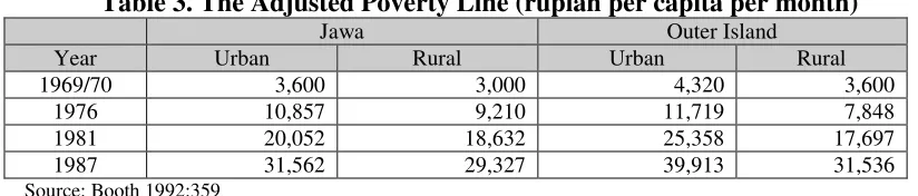
The actual poverty lines then were adjusted to 1976 and 1981 prices using the indexes

given in Asra (1989: Table 3). The result of adjustment is represented in table 3.

Table 3. The Adjusted Poverty Line (rupiah per capita per month)

Jawa Outer Island

Year Urban Rural Urban Rural

1969/70 3,600 3,000 4,320 3,600

1976 10,857 9,210 11,719 7,848

1981 20,052 18,632 25,358 17,697

1987 31,562 29,327 39,913 31,536

Source: Booth 1992:359

There are still several poverty lines summarized in Table 1. Basically, they can be

divided into two groups i.e. poverty lines based on ‘sufficient calorie/good’ and i.e. poverty

lines based on income/expenditure.

Urban-Rural Poverty Line

It is commonly believed that the living cost in urban area is higher than in rural area.

To take account the spatial difference in cost of living index, urban and rural poverty lines are

set separately. Therefore, to meet the same level of utility, urban people would need higher

expenditure than rural people. Some practical weaknesses still exist on setting different

comparisons in many countries. In many cases, regional poverty lines should be based only on

the FEI approximation. But if the urban-rural cost-of-living difference is large, then the FEI

approximation is a very misleading indicator.

According to Ravallion and Bidani (1994), there are several reasons why FEI can not

be a appropriate indicator for poverty comparisons. First, it is because the urban-rural prices

differ not only in nominal, but also in real terms. To that extent, the demand behaviors at

given real expenditure levels are also different. For example, the prices of some non-food

goods are lower (relative to foods) in urban areas. The food demand and FEI will then be

lower in the urban areas.

Second, the activities in typical urban jobs (e.g. factory works) tend to require fewer

calories than do rural activities (e.g. agricultural works). Finally, since tastes may differ,

urban households may have more expensive food tastes, but relatively lower calorie intake.

These three cases will result in less calorie expenditure for urban households. But clearly this

should not be taken as evidences of poverty.

Problems on measurement poverty line can also take place when there is mobility

across the groups being considered in the poverty line, such as migration from rural to urban

areas (see Ravallion 1992). Suppose someone who is just above the poverty line from the

rural area migrates to the urban area. If this person earns income gain (the income from

working in urban minus income in rural area) less than the difference in the urban-rural

poverty lines, then there will be an increase in poverty statistics. This may happen although

the person is actually better off in terms of living standards being used. In that case, an

economic development process that generates urban area enlargement may results in an

III. Methodology

The Linear Expenditure System (LES)

In this paper, it is assumed that the rural and urban people have a utility function

following the more general Cobb-Douglas. Stone (1954) made the first attempt to estimate a

system equation explicitly incorporating the budget constraint, namely the Linear Expenditure

System (LES).

Formally the individual household’s preferences defined on n goods are characterized

by a utility function of the Cobb-Douglas form. Klein and Rubin (1948) formulated the LES

as the most general linear formulation in prices and income satisfying the budget constraint,

homogeneity and Slutsky symmetry. Basically, Samuelson (1948) and Geary (1950), derived

that the LES representing the utility function:



x

x

 

x

x

 

x

x





x

x



x

x

U 1 2 3 n

n

1









 

 

 ………….(1)

The individual household’s problem is to choose xi that can maximize its utility U(xi)

subject to its budget constraint. Therefore, the optimal choice of xi is obtained as a solution to

the constrained optimization problem as follows:

Max





x

x

x

U i

n

1 i

i





 



xi

Subject to: PX  M

Solving the utility maximization problem, we can find the Marshallian (uncompensated)

demand function for each commodity xi as follows:

                 _n 1 i i i n 1 j o j j i o i i p x p x x

Where: i1,2,……..n j1,2,……..n

Since a restriction that the sum of parameters i equals to one,

1 n 1 i i   

, is imposed

equation (2) becomes:

p

x

p

x

x

M _

       







Equation (2) can be also reflected as the Linear Expenditure System as follows:

          





i

x

p

x

p

x

p

This equation system (4) can be interpreted as stating that expenditure on good i ,

given as pixi, can be broken down into two components. The first part is the expenditure on a

certain base amount xio of good i , which is the minimum expenditure to which the consumer

is committed (subsistence expenditure), pixio (Stone 1954). Samuelson (1948) interpreted xio

as a necessary set of goods resulting in an informal convention of viewing xio as non-negative

quantity. The restriction of xio to be non-negative values however is unnecessarily strict. The

utility function is still defined whenever:

_x

_x

necessary level of consumption is misleading (Pollak, 1968). The xio allowed to be negative

provides additional flexibility in allowing price-elastic goods. The usefulness of this

generality in price elasticity depends on the level of aggregation at which the system is

treated. The broader the category of goods, the more probable it is that the category would be

price elastic. Solari (in Howe 1954:13) interprets negativity of xio as superior or deluxe

In order to preserve the committed quantity interpretation of the xio’s when some xio

are negative, Solari (1971) redefines the quantity

_p

_x



as ‘augmented supernumerary

income’ (in contrast to the usual interpretation as supernumerary income, regardless of the

signs of the xio). Then, defining n* such that all goods with in* have positive xio and goods

for i>n* are superior with negative xio, Solari interprets

x p o j 1 j j n*  

as supernumerary income

and x p o j n 1 j j n*   

as fictitious income. The sum of ‘Solary-supernumerary income’ and

fictitious income equals augmented supernumerary income. Although somewhat convoluted,

these redefinition allow the interpretation of ‘Solari-supernumerary income’ as expenditure in

excess of the necessary to cover committed quantities.

The second part is a fraction i of the supernumerary income, defined as the income

above the ‘subsistence income’ _{p x}o j n 1 j j  

needed to purchase a base amount of all goods. The

i are scaled to sum to one to simplify the demand functions. The i is referred to as the

marginal budget share, i /i. It indicates the proportion in which the incremental income is

allocated.

The household’s food poverty line (FPL) for specific region j can be found by

summing up the minimum expenditure to which the consumer is committed (subsistence

expenditure). And then, the household poverty line (PL) for specific region j can be derived

(j is the contribution of FPL on PL for region j).





p

_x

PL

x

p

FPL

2







xo

The estimated Engel curve is estimated using all households i for each region j is presented

as:

u

FPL

e

log

j ij j

j

ij 

  

   









Where ij is the food share of total expenditure

eij is total expenditure

FPLj is the food poverty line for region j PLj is the poverty line for region j

j and j are parameter to estimated

IV. Data, Estimation, Result and Simulation

Data

This paper uses the secondary pooled data (time series and cross section data) about

individual household’s expenditure from Statistik Harga Pedesaan (Rural Price Statistics) and

Survey Biaya Hidup (Survey of Living Cost) published by the Central Bureau of Statistics

(Badan Pusat Statistik, BPS) Indonesia 1980, 1981, 1984, 1987, 1990, 1993 and 1996. The

data used are consumption on foods, prices of foods2, income (total expenditure) of household

by rural and urban households by provinces. This paper is based on ten food

commodity-groups: Cereals (X1), Tubers (X2), Fish (X3), Meat(X4), Eggs and Milk (X5), Vegetables

(X6), Nuts (X7), Fruits (X8), Prepared Foods (X9), Tobacco / Cigarette (X10). Computer

program Shazam version 8 is applied for estimating the parameters.

2

We will use the average of the price of commodity group:

n n

1 i ki k

p

p



The 26 provinces of Indonesia are grouped into 5 groups of region based on the

geography i.e. Java and Bali; Sumatra; Kalimantan; Sulawesi; and the rest of Indonesia. Some

problems faced about availability of prices data are overcome by interpolation.

Estimation

The estimation of a linear expenditure system (LES) shows certain complications

because, while it is linear in the variables, it is non-linear in the parameters, involving the

products of i and

x

i in equation systems (2) and (3). There are several approaches to

estimation of the system (see Intriligator, Baskin, Hsaio 1996). This paper applies one of the

approaches: selecting i and

x

i simultaneously by setting up a grid of possible values for the

2n-1 parameters (the –1 based on the fact that the i sum tends to unity, n ₁

1

i i







) and

obtaining that point on the grid where the total sum of squares over all goods and all

observations is minimized.

The reason is that when estimating a system of equation seemingly unrelated

regression (SUR), the estimation may be iterated. In this case, the initial estimation is done to

estimate variance. A new set of residuals is generated and used to estimate a new

variance-covariance matrix. The matrix is then used to compute a new set of parameter estimator. The

iteration proceeds until the parameters converge or until the maximum number of iteration

reached. When the random errors follows a multivariate normal distribution these estimators

will be the maximum likelihood estimators (Judge et al 1982:324).

Rewriting equation (4) to accommodate a sample t=1,2,3,…..T and 10 goods yields

e x p x p x p e x p x p x p e x p x p x p t 10 10 1 j o j j 10 o t 10 t 10 t 10 t 2 10 1 j o j j 2 o t 2 t 2 t 2 t 1 10 1 j o j j 1 o t 1 t 1 t 1 M t 10 .... ... ... ... ... ... ... .... ... ... ... ... ... ... M t 2 M t 1                                       

for all i and j …….……..…….(7)

Where: eit is error term equation (good) i at time t.

Given that the covariance matrix 

 

_e

_e

t

t where

e



e

e

e



'

t , ,... and  is not

diagonal matrix, this system can be viewed as a set of non-linear seemingly unrelated

regression (SUR) equations. There is an added complication, however. Because 10 _M

1 i it itx p   

the sum of the dependent variables is equal to one of the explanatory variables for all t, it can

be shown that



_e

_e

_e



estimation procedures. The problem is overcome by estimating only 9 of the ten equations,

say the first nine, and using the constraint that

1 10 1 i i   

, to obtain an estimate of the remaining

coefficient 10 (Barten, 1977).

The first nine equations were estimated using the data and the maximum likelihood

estimation procedure. The nature of the model provides some guide as to what might be good

starting values for an iterative algorithm3. Since the constraint the minimum observation of

expenditure on good i at time t (xit) greater than the minimum expenditure

x

satisfied, the minimum xit observation seems a reasonable starting value for

x

process. Also the average budget share,

           T 1 t t it it 1 M x p

T , is likely to be a good starting value for

i in the iterating process (Griffith et al, 1982). It is because the estimates of the budget share

i will not much differ with the average budget share. The estimate and statistical analysis is

presented in the Appendix.

Result

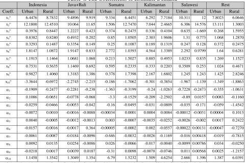
Table 4 represents the estimated parameters from linear expenditure equation system

(7). The parameters have both negative and positive signs. The negative value of xio seems to

break the restriction that xio should be positive because it reflects the minimum expenditure to

which consumer is committed (subsistence expenditure), Pixio (Stone 1954). In the same

sense, Samuelson (1948) defines xio as a necessary set of goods resulting in an informal

convention of viewing xio as a non-negative quantity. However, the restriction of xio to be

non-negative values, is unnecessarily strict because the utility function is still theoretically

defined whenever

_x

_x

i

i  (Howe 1954:13). Thus the interpretation of xi

o _{as a necessary}

level of consumption as being to some extent misleading (Pollak, 1968). The xio is allowed to

be negative provides additional flexibility in allowing price-elastic good4.

4_{The expression for own-price elasticity:}





x

x







x x

i o

i _ by the requirement (xi- xio )>0.

Since i >0 and 1

10

1 i i





p

p

x

x

p

p

x

x









Table 4. The Coefficients of Estimate Demand

Indonesia Java+Bali Sumatra Kalimantan Sulawesi Rest Coeff. Urban Rural Urban Rural Urban Rural Urban Rural Urban Rural Urban Rural

x1o 6.4476 8.7832 9.4896 9.919 9.334 6.4451 6.292 7.7184 10.311 12 7.8023 6.0646

x2o 12.1800 12.4510 10.064 11.65 1.506 12.7470 7.044 2.4665 6.306 14.576 13.111 1.3003

x3o 0.3976 0.8447 1.2227 0.423 0.374 0.2475 0.336 0.4104 0.635 -1.669 0.268 1.5955

x4o 0.8382 0.8240 0.4932 0.202 0.85 1.0505 2.303 1.9606 1.31 0.773 1.068 1.2870

x5o 0.3293 0.1487 0.3354 0.149 0.25 0.1087 0.189 0.1319 0.247 0.128 0.372 0.2475

x6o 1.8147 1.0872 1.9147 0.833 2.772 1.0393 4.564 1.3389 2.292 0.9799 1.64 0.6281

x7o 1.1915 1.1464 1.0681 1.068 0.213 1.5027 0.885 0.4953 1.0233 0.835 1.269 1.1527

x8o 0.7531 0.5635 1.1469 0.692 0.595 0.2335 0.333 0.2203 0.3509 0.253 1.024 0.4671

x9o 0.9827 1.4060 1.3183 1.386 0.378 1.7398 2.167 1.6802 1.245 1.243 1.425 2.8246

x10o -3.3644 -0.6972 -2.2745 -2.215 -0.186 -1.7062 -0.301 -0.3854 -1.967 -1.139 -1.349 -1.8863

1 -0.1909 -0.2477 -0.2281 -0.238 -1.363 -0.3199 -0.24 -1.0263 -0.7228 -0.2473 -0.355 -1.0631

2 0.1086 -0.0651 -0.0778 -0.068 -3.3 -0.1529 -0.209 -2.2502 -0.89 0.0157 0.0083 -0.1160

3 -0.0259 -0.0466 -0.0053 -0.042 -0.16 -0.0495 -0.031 -0.0809 -0.035 -0.171 -0.059 -1.4542

4 -0.0072 0.0010 -0.0016 -0.0088 -0.00034 0.0001 0.0004 0.0084 -0.00012 -0.0031 0.00004 0.1013

5 0.0040 -0.0005 -0.0012 -0.0013 0.003 -0.0007 -0.0035 -0.0252 -0.0026 -0.002 0.0017 0.2422

6 -0.0157 -0.0016 -0.0017 0.364 -0.00005 -0.0002 0.002 -0.0557 -0.00022 0.00131 -0.00047 -0.7270

7 -0.0061 -0.0087 -0.0184 -0.0096 -0.686 -0.0032 -0.0026 -0.1169 -0.016 0.00418 -0.019 -0.7815

8 0.0092 0.0135 0.0254 -0.0086 0.026 -0.0066 -0.017 -0.0040 -0.0099 0.00786 0.034 -0.0250

9 -0.0218 0.0017 0.0039 0.0187 -0.31 0.0098 -0.0078 -0.0746 0.011 0.00568 0.0025 -1.2157

10 1.1458 1.3542 1.3049 1.354 6.79 1.5232 1.509 4.6254 2.666 1.396 1.387 6.0391

Source: Statistik Harga Pedesaan (Rural Price Statistic) and Survey Biaya Hidup (Survey of Living Cost), BPS, calculated. Note: Statistical analysis is provided in Appendix C

The level of commodity aggregation could cause negative xio. Solary (in Howe

1954:13) interprets negativity of xio as superior or deluxe commodities. Superior

commodities can be ranked hierarchically with regard to

i o i i x

p _{. When total expenditure}

increase, superior goods enter the consumption pattern in order of increasing

i o i i x

p _.

Table 4 also shows that there are some negative value of i . The negative i means

that when there is an increase in income such that supernumerary income is negative

   

 

 



10

1 j

0 j

j 0

M p_x the demand for good i will decrease. Also, if there is an increase in income

such that supernumerary income is positive  _10 _ 

0

decrease. The negative value of i indicates that if there is an increase of income, the demand

for good i will decrease (inferior good). Good i is an inferior good. Two properties of LES are

that inferior and complementary are disallowed. Evaluation of the expression

p x

i i i

M



 _



reveals that, in the LES, the income elasticity is always positive, inferior goods are not

allowed. Cross substitution matrix are positive with LES. However, at the high the level of

aggregation employed in this study, this limitation is not restrictive. It would be possibly to

find the negative i, when a research is related with the aggregation data. In fact, the goods

could be normal or inferior good. Therefore, when we aggregate those goods the nature of the

goods (normal or inferior) will appear in the aggregate data. The higher level of aggregation,

the less likely it is that consumption of any given category would decline with an increase in

income, negative i (Howe 1974:18).

Based on these i and xio interpretations, in general tobacco/cigarette (x10) is superior

or deluxe (price-elastic) commodity in both rural and urban Indonesia, whereas the other

commodity groups are price-inelastic goods, except fish (x3) that is also a price-elastic good

for rural households in Sulawesi. It is shown by negative x10o for all regions and negative x3o

for rural Sulawesi respectively. Since food is a basic good (basic needs or necessity good), it

is theoretically believed that food would be inelastic. A household’s demand for food would

be not very responsive to the change in food prices. Tobacco/cigarette has a positive marginal

budget share, estimate 10 positive. It clearly means that when a household’s income

increases the demand for tobacco/cigarette (x10) also increases. The strange result is found in

rural Sulawesi where fish (x3) is a price-elastic good but has a negative marginal budget share.

From the structure of food consumption, in general a rural household’s minimum

consumption of cereals (x1), tubers (x2), fish (x3) is relatively much more than urban

household’s one. In contrast, urban household’s minimum consumption of meat (x4), egg and

milk (x5), vegetables (x6) and prepared foods (x9) is relatively higher than for a rural

household. However, the urban and rural households have relatively the same minimum

consumption of nuts (x7) and fruits (x8).

Why do some of these coefficients differ from staples across region ad rural-urban

areas? The deep research is needed to answer this question. Some general factors could be

addressed in explaining the difference (Widodo, 2000). Elaine (1999) notes that there are 5

factors affecting food decisions made by individual consumers i.e. food availability, cultural

factors, psychological factors, lifestyle factors and food trends.

First, food availability is the crucial factor in determining food consumption. It is

obvious that households will consume relatively more a kind of food that is abundant in that

area. Second, food habits are culture factors that make an important contribution to the food

decisions consumers make. Although some view and food habits as unchanging and static, it

is now known that they are continually changing as they assimilate to immigration, travel and

socio-economic environment (Jerome, 1982; Lowenberg et al., 1974: Senauer et al., 1991;

Kittler and Sucher, 1995). However, there are certain elements of food habits that might be

difficult to change, such as the concept of meals, meal patterns, the number of meals eaten in

a day, when to eat what during the day, how food is acquire and prepared, the etiquette of

eating and what is considered edible as food (Elaine, H. 1999:288).

Third, psychological factors consist of food preferences, food likes and dislikes and

give an indication of the amount of satisfaction an individual anticipates from eating a food.

Food preference is a result of physiological and psychological development and social

experiences, and is related to degree of liking a food (Elaine, H. 1999:289). Liked foods are

those that are familiar, considered pleasant, and are usually the ones eaten, thus food

preference predict consumption. In contrast, disliked foods are rejected either because they

are considered unpleasant or they are unfamiliar foods that have never been tasted.

Fourth, lifestyle factors. Lifestyles describe how people seek to express their identity

in many areas, including food selection. Fifth, food trends. Several established and emerging

food trends identified by Sloan (1994, 1996, and 1998) affect the food decisions individual

make. These include foods that are fresh; quick to cook; ethnic with distinctive ingredients,

favour and spices; fusion foods (the combine ethnic cuisines); less meat; more vegetarian

meals; labelled natural organic; available in a variety of places; health promote; and physical

performance-enhancing energy foods.

Simulation

The economic crisis happened since 1996 has caused some increases in price of foods

and decrease in income. This paper utilizes some figures from the previous other researches

and surveys. Two settings based on those can be withdrawn. The increase of prices (inflation)

from the BPS and also the inflation level suggested by IFLS (Indonesia Family Life Survey)

will be used i.e. inflation per province inflated from the BPS by 14% for urban and 16% for

rural. This paper assumes that the inflation rate per province reflects the food inflation rate in

that province. This assumption is taken because the data of inflation rate of each commodity

groups per province is unavailable. Therefore, the shortcoming of this assumption is that all

avoided if the data inflation rate of each commodity group per province can be reached. It

gives opportunities to other researchers to do some simulation based on the available data.

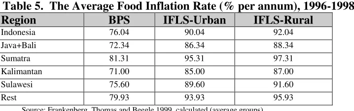
Table 5 represents the calculated unweighted average food inflation rate in each

considered region5. The second column consists of the average inflation rate for each region

calculated from taking the average of inflation in all provinces published by the BPS. For

example, according to BPS the food prices increase by 76.04% during 1996-1998 period.

Unfortunately, the BPS does not distinguish the inflation rate in urban and rural areas.

Therefore, it is assumed that rural and urban areas have the same inflation rate in this study in

one part. In fact, urban and rural have obviously different rates of inflation.

Table 5. The Average Food Inflation Rate (% per annum), 1996-1998

Region BPS IFLS-Urban IFLS-Rural

Indonesia 76.04 90.04 92.04

Java+Bali 72.34 86.34 88.34

Sumatra 81.31 95.31 97.31

Kalimantan 71.00 85.00 87.00

Sulawesi 75.60 89.60 91.60

Rest 79.93 93.93 95.93

Source: Frankenberg, Thomas and Beegle 1999, calculated (average groups)

The IFLS data suggests that inflation between the rounds of the survey has been about

15% higher than the rate estimated from BPS data (Frankenberg, Thomas, Beegle 1999:14)

and therefore IFLS suggests to inflate the BPS inflation by 14% for urban and 16% for rural

household. The third and fourth columns of Table 5 represent urban and rural average

inflation rates respectively suggested by the IFLS for each region. These inflation rates (we

5_{The unweighted average inflation rate per province is calculated by applying formula as follows:}

n n

1

j j

i



 _  where i is

call as BPS scenario and IFLS adjusted scenario) will be used to inflate the prices, therefore

the prices pre-crisis and post-crisis can be withdrawn.

a. Households’ Food Poverty Line (FPL)

The subsistence (minimum) expenditure can virtually be used to derive the food

poverty line (FPL). Therefore, by applying equation 5 and some scenarios about prices

explained above, the household poverty lines can be calculated. Table 6 shows the food

poverty line (FPL) defined from this paper for 1980-1998. These figures are derived from

summing up of the multiplication of estimated minimum consumption (xio) (from Table 4)

and their respective prices, so that we get the total minimum (subsistence) expenditure for

food as the food poverty line.

Table 6. The Food Poverty Line (Rp/household/month)

Region Indonesia Java+Bali Sumatra Kalimantan Sulawesi Rest

URBAN

1980 11,625 6,639 13,223 17,513 8,540 8,243 1981 12,246 7,293 13,586 19,005 9,004 8,781 1984 14,322 9,434 14,938 23,311 11,008 10,406 1987 17,212 12,408 16,710 29,288 13,921 12,516 1990 21,105 16,172 19,243 36,895 18,002 15,463 1993 25,939 20,162 21,736 48,899 23,034 20,210 (before crisis) 1996 31,884 24,561 26,632 65,657 32,207 28,730 (after crisis IFLS adj) 1998 60,495 45,767 52,014 121,466 61,064 55,716 (after crisis BPS) 1998 56,032 42,329 48,286 112,274 56,555 51,694

RURAL

In general, the poverty lines in urban areas are greater than in rural areas. In

Indonesian urban areas, before crisis (1996) it was Rp 31,884 per month, and then, (1998) it

became Rp 60,495 per month under IFLS adjusted scenario or Rp 56,032 per month under

BPS scenario after crisis. Meanwhile in Indonesian urban areas, before crisis (1996) it was Rp

26,656 per month, and then, (1998) it became Rp 51,110 per month under IFLS adjusted

scenario or Rp 48,845 per month under BPS scenario after crisis.

Both urban and rural poverty lines in Kalimantan is higher than in other regions. It

could be caused by two virtual reasons. First, the food poverty line extremely depends on the

level of prices. In fact, the levels of prices in Kalimantan are relatively higher than the other

regions. Second, the food habits in term of kinds of food consumed are also effect on the food

poverty line. Determining the kind and amount of food included in the food poverty lines

calculation are difficult. This paper has advantage in determining the amount of each food

consumed (as presented in Table 4). The Kalimantan households eat relatively more

expensive food (such as meat (x4o) and prepared food (x9o)).

b. Poverty Line

People consume food and non-food. Therefore, the food poverty line is only one part

of poverty line. The second one is non-food poverty line. Determining the non-food poverty

line is more complex than the food poverty line. Establishing the allowance made for the

non-food expenditure is more difficult, because there is no equivalent of a nutritional standard to

provide even a weak anchor to the amount (Pradhan 2000):6). In this paper, the non-food

consumption (equation 6). The non-food component of the poverty line is set at the expected

non-food consumption for those whose total consumption equals the food poverty line.

Table 7. The estimate of Parameter j

Regions (j) Urban Rural

Indonesia 0.552 * (0.006) 0.611* (0.005) Java+Bali 0.574* (0.021) 0.602* (0.035) Sumatra 0.565* (0.11) 0.612* (0.009) Kalimantan 0.539* (0.009) 0.567* (0.012) Sulawesi 0.615* (0.025) 0.651* (0.015) Rest of Indonesia 0.543* (0.017) 0.657* (0.014) Note: Standard error in parentheses (). * significant at 1% level of significance

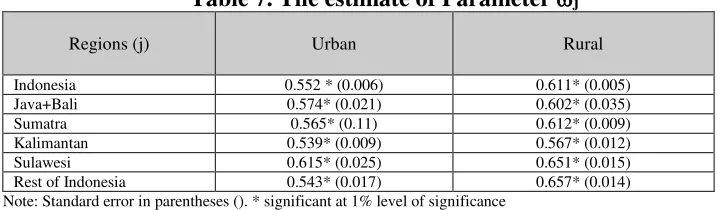
Table 7 shows the estimate parameters in equation 6. Statistically, they are significant

at 1% level of significance. The food share of total expenditure in every region is greater than

50 percent. It means that more than half of total expenditure is spent for food consumption.

As commonly believed, the urban food share of total expenditure in every region is smaller

than the rural one. It implies that urban households spend their total expenditure in the smaller

proportion on food than rural households do.

Table 8 presents the poverty line derived. It is easy to understand that the method used

to derive such households’ poverty lines is extremely depends on the food poverty lines and

the food share derived above. Regions whose have higher food poverty line and smaller

proportion of food tend to have higher poverty line. In contrast, regions whose have lower

food poverty line and higher proportion of food tend to have lower poverty line. Therefore, all

factors effecting the food poverty line and the food share (such as food habits, religion,

culture, belief, climate, and season) have brought some differences in the poverty line across

Table 8. The Households’ Poverty Line (Rp/household/month)

Region Indonesia Java+Bali Sumatra Kalimantan Sulawesi Rest URBAN

1980 16,833 9,467 18,975 25,586 11,828 12,010 1981 17,732 10,400 19,496 27,766 12,471 12,794 1984 20,738 13,453 21,436 34,057 15,246 15,162 1987 24,923 17,694 23,979 42,790 19,281 18,236 1990 30,560 23,061 27,614 53,904 24,933 22,530 1993 37,560 28,751 31,191 71,441 31,902 29,446 (before crisis) 1996 46,168 35,024 38,217 95,925 44,607 41,860 (after crisis IFLS adj) 1998 87,597 65,264 74,640 177,462 84,574 81,178 (after crisis BPS) 1998 81,134 60,361 69,290 164,032 78,329 75,318

RURAL

1980 14,314 5,842 17,342 21,964 8,224 9,617 1981 15,055 6,385 17,839 23,670 8,789 10,246 1984 17,568 8,243 19,467 29,408 10,757 12,330 1987 21,070 10,882 21,581 37,258 13,638 15,085 1990 25,819 14,383 24,684 47,071 17,824 18,735 1993 31,541 17,704 27,759 62,854 22,955 24,710 (before crisis) 1996 37,025 21,276 31,866 81,109 31,685 35,444 (after crisis IFLS adj) 1998 70,992 40,072 62,875 151,674 60,709 69,447 (after crisis BPS) 1998 65,068 36,668 57,777 138,697 55,640 63,776

Source: Statistik Harga Pedesaan (Rural Price Statistic) Survey Biaya Hidup (Survey of Living Cost), BPS, calculated.

V. Conclusion

Increase in food prices due to economic crisis has increased the minimum

(subsistence) food expenditure defined as the food poverty line (FPL) of both urban and rural

people. During 1996-1998, the increase in the subsistence food expenditure was averagely

more than doubled. Therefore, it is clear that the share of food expenditure on the total

expenditure of urban and rural household increased drastically.

The alternative measurement of food poverty line can also be derived from the

consumption theory namely Linear Expenditure System (LES). This method has more

advantage in determining the amount of good consumed that is core problem in establishing

conclude that the economic crisis has effected the urban poverty line increasing sharper than

the rural one.

References

Ariffin, J. (ed.), 1994. Poverty Amidst Plenty, Petaling Jaya, Malaysia: Pelanduk.

Asra, Abuzar, 1989. ‘Inequality trends in Indonesia, e re-examination’. Buletin of Indonesian Economic Strudies. 25(2):100-10.

Asra, Abuzar, 1999. ‘Rural-urban differences in cost of living and their impact on poverty

measures. Buletin of Indonesian Economies. Vol. 35 no. 3, December.

Asra, Abuzar, and Vivian S.F. 2001. Poverty Line: Eight Countries’ Experiences and the

Issue of Specificity and Consistency. A paper was delivered at the Asia and Pacific

Forum of Poverty: Reforming Policies and Institutions for Poverty Reduction. ADB.

Manila. 5-9 February.

Barten, A.P., 1977.’The system of consumer demand function approach: a review’.

Econometrica 45:23-51. Also in M.D. Intriligator, Ed., Frontier of Quantitative

Economics, Vol.3. Amsterdam:North-Holland Publishing Company.

Booth, A., 1999a. ‘The Impact of the Crisis on Poverty and Equity’, in Arndt and Hill (1999).

Booth, A.,1999b. ‘The Social Impact of the Asian Crisis: What Do We Know Two Years

On?’, mimeo.

Booth, A., 1993. ‘Counting the Poor in Indonesia’, Bulletin of Indonesian Economic Studies,

v.29/1.

Booth, A., 1992. The oil Boom and After: Indonesian Economic Policy and Performance in

the Soeharto Era. Oxford University Press.

BPS . 1998. Crisis, Poverty and Human Development in Indonesia 1998, Jakarta.

Deaton A.S. and J. Muellbauer., 1980. Economic and Consumer Behaviour. Cambridge:

Deaton A.S. and J. Muellbauer., 1986. ‘Demand analysis’. in Z. Griliches and M.D.

Intriligator, Ed, Handbook of Econometrics, Vol. 2. Amsterdam: Norh-Holland

Publishing Company.

Dhanani, S. and I. Islam, 2000. Poverty, Inequality and Social Protection: Lessons from the

Indonesian Crisis.Jakarta: UNSFIR.

Elaine, H., 1999.’Factors affecting food decisions made by individual consumers’. Food Policy. Vol. 24: 287-94.

Fields, G.S., 1993. ‘Poverty and Income Distribution: Data for Measuring Poverty and

Inequality Changes in the Developing Countries’, Journal of Development

Economics, v.44.

Foster, J. et al., 1984. ‘A Class of Decomposable Poverty Measures’, Econometrica, v.52/3.

Frankenberg,E., Thomas, D. and Beegle, K., 1999. The Real Cost of Indonesia’s Economic

Crisis: Preliminary Findings from the Indonesia Family Life Survey. Labour and

Population Program Working Paper Series 99-04.

Griffiths, W., R.C. Hill and G.G. Judge, 1993. Learning and Practicing Econometrics. John

Wiley and Sons, Inc. Canada.

Howe, H., 1974. Estimation of the linear and quadratic expenditure systems: A cross-section

case for Colombia. University Microfilm Internatinal, Ann Arbor, Michigan, USA,

London, Engalnd.

ILO/UNDP., 1998. Employment Challenges of the Indonesian Economic Crisis, Jakarta.

Intriligator, M.D., Bodkin, R.G. and Hsiao,C., 1996. Econometric Models, Techniques, and

Applications. Prentice–Hall Inc, Upper Saddle River, NJ 07458.

Jerome, N.W., 1982. ‘Dietary patterning and change: a continuos process’. Contemporary Nutrition Newsletter. 7(6), General Mills, Inc.

Joseph, P., 1968. ‘Application of linear expenditure system to NSS data some further result,’

Economic and Political Weekly. April 13.

Judge, G.G., Hill. R.C., Griffiths. W.E. Helmut,L., and Lee.T.C., 1982. Introduction to the

Klein, L.R., and Rubin, H., 1948. ‘A constant utility index of the cost of living’. Review of Economic Studies. XV(2). No. 38: 84-87.

Lowenberg, M.E., Thodunter, E.N., Wilson, E.D., Savage, J.R., Lubawski, J.L., 1974. Food

and Man, 2nd ed. John Wiley and Sons, New York.

McNamara, R.S., 1972. Address to Board of Governors. Washington D.C. World Bank,

September 25.

Meier, G.M.,1995. Leading Issues in Economic Development. Six Edition. Oxford University

Press.

Philips, L., 1993. Applied Consumption Analysis. Revised and enlarged ed. Amsterdam:

North Holland Publishing Company.

Pollak, R.A., 1968. ‘Additive utility function and linear Engel curves’. Discussion Paper. No 53, Department of Economics, University of Pennsylvania, revised Feb.

Pradhan, M. et al., 2000. ‘Measurements of Poverty in Indonesia: 1996, 1999, and Beyond’,

SMERU Working Paper, 6/00.

Ranjan, R. 1985. ‘A dynamic analysis of expenditure pattern in rural India’. Journal of Development Economics. Vol. 19.

Ravallion, M. (1992). Poverty Comparison: A Guide to Concepts and Methods, Washington,

D.C.: The World Bank.

Ravallion, M. and B. Bidani, 1994. ‘How Robust Is a Poverty Profile?’, The World Bank Economic Review, v.8/1.

Rein, M., 1970. ‘Problems in the Definition and Measurement of Poverty’, in Townsend

(1970).

Samuelson, P.A. , 1948. ‘Some implication of linearity’. Review of Economic Studies. XV (2). No. 38: 88-90

Satish, R. and Sanjib, P., 1999. ‘An analysis of consumption expenditure of rural and urban

income groups in LES framework. ASIAN Economies.

Sen, A.K., 1999. Development as Freedom, New York: Alfred A. Knopf.

Sen, A.K., 1992. Inequality Reexamined, New York: Oxford.

Sen, A.K., 1981. Poverty and Famines: An Essay on Entitlement and Deprivation, New York:

Oxford.

Sen, A.K., 1976. ‘Poverty: An Ordinal Approach to Measurement’, Econometrica, v.44/2.

Suharyadi, A. et al., 2000. ‘The Evolution of Poverty During the Crisis in Indonesia, 1996 to

1999 (Using Full SUSENAS Sample)’, SMERU Working Paper, 3/00.

Suharyadi, A. et al., 1999a. ‘Update on the Impact of the Indonesian Crisis on Consumption

Expenditures and Poverty Incidence: Results from the December 1998 Round of 100

Villages Survey’, SMERU Working Paper, 8/99.

Suharyadi, A. et al., 1999b. ‘Poverty Measurement in Indonesia: Comparisons Over Time

(1996 to 1999) and Across Regions’, paper presented at the “International

Conference on Methodologies of Poverty Calculation in Indonesia”, Jakarta.

Sutanto, A., 1999a. ‘The December 1998 Poverty Estimate: Methodological Issues’, paper

presented at the “Workshop on Poverty Number Computational Method”, Jakarta.

Sutanto, A.,1999b. ‘The December 1998 Poverty in Indonesia: Some Findings and

Interpretation’, paper presented at the “Round Table discussion on Number of

Indonesia Poor People (Method and Forecasting)”, Jakarta.

Sutanto, A., A. et al. (1999). ‘Poverty Measurement: Problems and Developmenrt’, paper

presented at the “International Conference on Methodologies of Poverty Calculation

in Indonesia”, Jakarta.

Solari, L., 1971. Théorie des Choix et Fonctions de Consommation Semi-Agrégées: Modéles

Statiques. Genéve: Librairie Droz: 59-63.

Stone, R., 1954. ‘Linear expenditure system and demand analysis: an application to the pattern of Britissh demand.’ Economic Journal. 64:511-27.

The Central Bureau of Statistics (Badan Pusat Statistik, BPS) of Indonesia, 1980, 1981, 1984,

1987, 1990, 1993, 1996. Statistik Harga Konsumen Pedesaan Di Java Dan Sepuluh

Provinsi Luar Java (Rural Consumer Price Statistics in Java and Ten Provinces Out

The Central Bureau of Statistics (Badan Pusat Statistik, BPS) of Indonesia, 1980, 1981, 1984,

1987, 1990, 1993, 1996. Survey Biaya Hidup (Survey of Living Cost) . Jakarta.

Townsend, P., 1979. Poverty in the United Kingdom, New York: Penguin Books.

World Bank, 1998. Indonesia in Crisis: A Macroeconomic Update, Washington.

Widodo, H.S.T., 2000. Indikator Ekonomi Dasar Perhitungan Perekonomian Indonesia.

Penerbit Kanisius, Yogyakarta.

Widodo, T., 2000. The Impact Of Economic Crisis On Rural And Urban Households: A Case

Study Of Indonesia. Research paper of The Australian National University.

Unpublished.

Widodo, T., 2002. The Household Poverty Line under LES Framework. Project Grant of

QUE-DEED, Gadjah Mada University. Unpublished.

Widyanti, W., Sudarno, S. and Asep, S., 2001. Short-term Poverty Dynamics: Evidence from

Appendix: Statistical Analysis

1. Testing for Contemporaneous correlation

If there contemporaneous correlation does not exist, the least square (OLS) rule separately to each equation is fully efficient an the there is no need to apply the seemingly unrelated regression (SUR) (Griffiths 1993:561). Therefore, if there is uncertainty concerning this proposition, it is useful to test whether the contemporaneous covariance are zero.

Ho: 21 = 31 = 32= …………= 98 =0 (or ij=0 for all ij)

H1: at least one covariance is non-zero

The appropriate test statistic, under the normal linear model, is given by:



_r

_r

_r

_r



98 2 32 2 31 2

21 ...

T    

 

where is the squared correlation

       jj ii 2 ij

r2ij

and









T i

i i

ij xb y xb

y j j j

'

  

 .

Table A.1. Contemporaneous Test for the ‘Average’ and ‘Poorest’ Households

No Regions  Decisions

Average Household

1 Urban Indonesia 1.215E+07 Reject Ho and conclude there is Contemporaneous 2 Rural Indonesia 2.442E+07 Reject Ho and conclude there is Contemporaneous 3 Urban Java+Bali 2.503E+06 Reject Ho and conclude there is Contemporaneous 4 Rural Java+Bali 4.076E+06 Reject Ho and conclude there is Contemporaneous 5 Urban Sumatra 2.205E+07 Reject Ho and conclude there is Contemporaneous 6 Rural Sumatra 4.447E+06 Reject Ho and conclude there is Contemporaneous 7 Urban Kalimantan 1.655E+07 Reject Ho and conclude there is Contemporaneous 8 Rural Kalimantan 2.653E+07 Reject Ho and conclude there is Contemporaneous 9 Urban Sulawesi 1.763E+07 Reject Ho and conclude there is Contemporaneous 10 Rural Sulawesi 4.664E+06 Reject Ho and conclude there is Contemporaneous 11 Urban Rest 7.449E+06 Reject Ho and conclude there is Contemporaneous 12 Rural Rest 1.297E+09 Reject Ho and conclude there is Contemporaneous

Under Ho, the test statistic  has an asymptotic 2-distribution with N(N-1)/2 (in our case

9(9-1)/2=36) degree of freedom, where N is the number of equations and the estimated error correlation are used in the computation of . The null hypothesis is rejected if  is greater than the critical value for a 2

(36)-distribution at pre-specified significance level.

At significance levels =1%, =5% and =10% the critical values 2

(36) are about

63.6907; 55.7585 and 51.8050 respectively. The calculated  and the decision about the contemporaneous correlation test for each region are presented in Table A.3.

2. Testing for significance of the coefficient estimate:

When error term e is not normally distributed, or independent variable X is random, we

have to refer to large sample distributions. We assume that X’X/T converges to a finite

non-singular matrix xx, and that X, if it is random, is at least contemporaneously

uncorrelated with error term e (Griffiths 1993:453). The estimate bk will be normally

 

var

bk k

 





The large sample theory suggests that normal distribution not the t-distribution should be used. The appropriate test is:

Ho: k=0

H1: k0

The calculated t-statistic is:

 

t

b

var

b

 

The null hypothesis is rejected if t-statistic is greater than the critical value for a N(0,1) distribution at pre-specified significance level. At significance levels =1%, =5%,

=10%, =15% and =20%, the critical values N(0,1) are about 2.57; 1.96; 1.65; 1.44 and 1.28 respectively. Tables below represent the significance test of each estimate parameters for each region:

* significant at level of significance, =1%, ** significant at =5%,

*** significant at =10%, **** significant at =15%, ***** significant at =20%.

INDONESIA JAVA+BALI

URBAN RURAL URBAN RURAL

Paramete rs

Coeff. Std. Error t-ratio Coeff. Std. Error t-ratio Coeff. Std. Error t-ratio Coeff. Std. Error t-ratio

x1o 6.4476* 1.0000 6.4475 8.7832* 1.0754 8.1676 9.4896* 1.0526 9.0153 9.9191* 1.0007 9.9117

x2o 12.1800* 0.6914 17.6150 12.4510* 0.6384 19.5030 10.0640* 0.6313 15.9430 11.6500* 0.6457 18.0420

x3o 0.3976** 0.1905 2.0869 0.8447** 0.4342 1.9454 1.2227* 0.1480 8.2599 0.4230 0.2590 1.6333

x4o 0.8382* 0.0626 13.3880 0.8240* 0.0613 13.4430 0.4932* 0.0446 11.0590 0.2018* 0.0550 3.6705

x5o 0.3293* 0.0218 15.1300 0.1487* 0.0137 10.8460 0.3354* 0.0318 10.5400 0.1493* 0.0197 7.5981

x6o 1.8147* 0.0986 18.4050 1.0872* 0.0781 13.9220 1.9147* 0.0727 26.3460 0.8332* 0.0782 10.6570

x7o 1.1915* 0.1074 11.0940 1.1464* 0.0833 13.7620 1.0681* 0.0985 10.8480 1.0684* 0.0671 15.9320

x8o 0.7531* 0.0595 12.6600 0.5635* 0.0555 10.1510 1.1469* 0.0821 13.9770 0.6922* 0.0958 7.2262

x9o 0.9827* 0.0716 13.7230 1.4060* 0.0639 21.9910 1.3183* 0.0952 13.8470 1.3864* 0.1170 11.8460

x10o -3.3644* 0.2841 -11.8420 -0.7***** 0.5341 -1.3054 -2.2745** 1.0868 -2.0928 -2.2148* 0.2862 -7.7393

1 -0.1909* 0.0612 -3.1168 -0.2477* 0.0346 -7.1632 -0.2281* 0.0408 -5.5943 -0.2382* 0.0622 -3.8276

2 0.1086*** 0.0685 1.5842 -0.0651 0.0613 -1.0614 -0.08**** 0.0521 -1.4920 -0.0679 0.0613 -1.1074

3 -0.0259** 0.0112 -2.3053 -0.0466** 0.0232 -2.0090 -0.005**** 0.0035 -1.5049 -0.0421* 0.0067 -6.2481

4 -0.0072 0.0096 -0.7492 0.0010 0.0054 0.1823 -0.0016 0.0050 -0.3195 -0.0088 0.0080 -1.0990

5 0.0040 0.0037 1.0760 -0.0005 0.0022 -0.2465 -0.0012 0.0037 -0.3288 -0.0013 0.0021 -0.6240

6 -0.0157 0.0132 -1.1919 -0.0016 0.0049 -0.3259 -0.0017 0.0058 -0.2985 0.0036 0.0060 0.6042

7 -0.0061 0.0213 -0.2856 -0.0087 0.0143 -0.6096 -0.018**** 0.0116 -1.5855 -0.0096 0.0104 -0.9251

8 0.0092 0.0126 0.7267 0.0135** 0.0058 2.3085 0.0254** 0.0104 2.4366 -0.0086 0.0141 -0.6074

9 -0.0218 0.0231 -0.9423 0.0017 0.0088 0.1887 0.0039 0.0118 0.3297 0.0187 0.0193 0.9714

10 1.1458* 0.1368 8.3745 1.3542* 0.0826 16.3943 1.3049* 0.0784 16.6501 1.354* 0.0870 15.5634