International Journal of Computer Applications (0975 – 8887) Volume 41– No.10, March 2012
22
Image Super-Resolution Reconstruction based on
Multi-Groups of Coupled Dictionary and Alternative
Learning
Sun Guangling
School of Communication and Information Engineering
Shanghai University China
200072
Li Guoqing
School of Communication and Information Engineering
Shanghai University China
200072
Jiang Xiaoqing
School of Communication and Information Engineering
Shanghai University China
200072
ABSTRACT
A novel image super-resolution reconstruction framework
based on multi-groups of coupled dictionary and alternative
learning is investigated in this paper. In dictionary learning
phase, each image of a training image set is taken as high
resolution image (HRI), the reduced and re-enlarged result of
HRI by interpolation is taken as low resolution image (LRI),
and the difference between them is residual image. To obtain
the mapping between residual and LRI, coupled dictionaries
are learned from joint data composed of residual image patch
and LRI patch features. Considering that distinguished texture
and structural characteristics reflected in image patches and
dictionary learning efficiency as well, multi-groups of coupled
dictionary and alternative learning scheme are proposed. In
reconstruction phase, LRI is obtained first. Then sparse
representations and corresponding errors are calculated for
each patch of the LRI by using low resolution component of
each group of coupled dictionary. The residual component of
coupled dictionary with minimum errors is applied to
reconstruct the corresponding residual image patch. All such
reconstructed residual patches compose a residual image.
Finally, the residual image and the LRI are fused to produce an
expected HRI. An experimental study is performed to
establish that the proposed approach improves the
super-resolution reconstruction quality.
Keywords
super-resolution, sparse representation, multi-dictionary,
alternative learning, principal subspace, orthogonal Gaussian
mixture model
1.
INTRODUCTION
Image Super-Resolution reconstruction (SR), as one of the
most valuable research topics, its aims is to get beyond the
resolution of imaging sensors or obtain a higher resolution
image. It has a variety of useful applications. Usually, a
high-resolution image is reconstructed from one or multiple
low-resolution images. If multiple low-resolution images are
available, they are registered at sub-pixel accuracy and a
higher resolution image is generated by reconstruction or
interpolation. However, with the expected scale of super
resolution is enlarged, the performance of SR will decay even
if the number of low-resolution image is increased. In a word,
when a large SR scale is required or low-resolution images are
insufficient, SR only using low-resolution images will easily
fail.
To break the limitation, numerous learning based schemes
have been proposed in recent years. Relying on the learned
prior knowledge, the SR reconstruction performed well
whereas the low-resolution image number is reduced
significantly even only a single low-resolution image is
available. In fact, learning based schemes have been well
popular in super-resolution and other image processing tasks.
The crucial point of it is to learn a mapping between low
frequency and high frequency and the learned mapping is
adopted to obtain the high-resolution image given a
low-resolution image. Freeman proposed the example-based
method [1]. As one of the earliest learning-based SR
reconstruction approaches, it modeled the spatial relations of
probability matrix between high resolution image patches or
high and low resolution image patches. Rich high frequency
information thereafter was estimated relying on the learned
matrix. However, the training images must be selected
carefully. In addition, the method is sensitive to noise and the
learning efficiency is relative low. Chang proposed neighbor
embedding [2]. It is assumed that corresponding high and low
resolution patches have same local geometrical manifold. First,
low and high dimensional manifolds were learned. Then
k-nearest neighbor representations of a low resolution patch
were searched in low dimensional manifold, and the weighted
representations and high dimensional manifold are used to
reconstruct the high resolution patch. But for low and high
resolution patches, the neighbor relations would not always be
preserved. To overcome the limitation, Chan improved
neighbor embedding from several respects, such as residual
neighbor embedding [3], edge detection and feature selection
[4].Compared to the example-based method, neighbor
embedding required less training samples and is less sensitive
to noise. Ni proposed a SR method based on Super Vector
Regression (SVR) [5]. By integrating additional constraints,
they transformed the kernel learning from a positive
semi-definite programming problem into a quadratic linear
programming problem. In this method, samples were selected
automatically and training set was not large. Moreover, it was
effective in both spatial and DCT domain. The robustness to
noise present in image was an advantage of this method.
Nevertheless, the high computation complexity of non-linear
SVR prohibits SR task with large-scale images.
Recently, sparse representation and dictionary learning have
become one of the most important tools to address a wide
range of image processing problems including super
resolution. Yang calculated sparse representations for raw
image patches [6]. In learning phase, they sampled a large
amount of pairs of image patches randomly from an outer
image set. Joint features composed of low and high features
extracted from high and low resolution patches were directly
used as a pair of redundant dictionary. In reconstruction phase,
features were extracted from low resolution image and its
sparse representations were applied with high part of the
redundant dictionary to recover a high resolution image patch.
Since the sparse coding was determined accordingly through
algorithm, it is not necessary to set the element number in
advance whereas the neighbor size must be set in neighbor
embedding. Compared with directly using image patched as a
dictionary, Yang improved his own method by learning a
dictionary to generate a more compact representation of patch
pairs, reducing the calculation complexity significantly [7].
Yang‘s work, which first applied sparse representation in
image super resolution, is a pioneer research in related field.
However, because of the large variation of data, a single
dictionary is not capable of representing data sparsely with a
high precision. In addition, Lagrange Dual and Lasso of
which efficiency were not satisfied were adopted to learn the
dictionary. Again in framework of sparse representation,
Zeyde proposed to train dictionary from the low resolution
input image itself [8]. Unlike the strategy of joint dictionary
learning proposed by Yang, Zeyde first learned the low
resolution dictionary using K-SVD algorithm [9] and then
obtained the high resolution dictionary with MOD algorithm
[10]. Although both learning efficiency and reconstruction
quality were improved, the method still learned a single
dictionary and a dictionary must be relearned for each input
low resolution image which undoubtedly dropped the
reconstruction efficiency. Moreover, the heavy computation
burden of K-SVD is also an annoying problem. Yang
proposed SVR integrated with sparse representations [11].
The support vector repressors and image patch category were
two crucial factors of this work and the computation
complexity of it is substantially reduced than that of existing
SVR based methods.
To overcome the previous drawbacks in sparse representation
framework, we propose multi-groups of coupled dictionary
and its alternative learning algorithm. Our first contribution is
the multi-groups of dictionaries. In principal subspace of low
resolution features, Orthogonal Gaussian Mixture Models
(OGMM) [12] is used to classify the low resolution image
patch automatically according to their features. In a sequel, a
coupled dictionary is learned by using low and high resolution
patches in respective patch category space so that multiple
coupled dictionaries are produced. During reconstruction, the
sparse representations and reconstruction error of low
resolution patch corresponding to low part of each coupled
dictionary are calculated. Next, the high resolution patch is
recovered using the calculated sparse representations and high
part of the coupled dictionary that has least reconstruction
error. In a brief, high frequency is complemented adaptively
International Journal of Computer Applications (0975 – 8887) Volume 41– No.10, March 2012
24 the alternative learning of coupled dictionary. Alternative
learning use low and high resolution data alternatively and
MOD algorithm to guarantee low and high resolution
dictionary are synchronized. At the same time, the learning
efficiency is also improved greatly.
2.
FRAMEWORK AND ALGORITHM
OF MULTI-DICTIONARY SCHEME
Statistics learning theory [13] shows that a dramatic augmentof training sample amount will definitely enhance the
generalization of dictionary. However, the variation of data
will also enlarge with many types of textures and edges
appearing. Clearly, a single dictionary is not sufficient to
represent data both sparsely and accurately. In other words,
single dictionary is under-fitting. Hence, data is categorized
into multiple groups based on its visual characteristics. After
that, dictionary is learned in respective data group. This
strategy will effectively reduce the bias of reconstruction error
with sparse representation and considerably boost the overall
performance of dictionary.
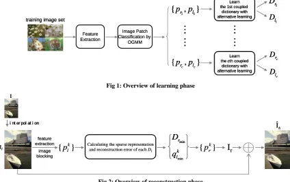
The framework consists of two phases: learning phase and
reconstruction phase, which have been shown in Fig 1 and Fig
2 respectively. In learning stage, we randomly sample a large
number of image patches from the low resolution images and
residual images at corresponding positions, which residual
image is difference between high resolution and low
resolution image. Then, features are extracted from the
residual and low resolution image jointly written as {pr, pl}. pl
is used and clustered by solving OGMM, generating
multi-groups of data. Upon each group of data, a coupled
dictionary composed of residual part Dr and low-resolution
part Dl is learned with alternative learning. In reconstruction
phase, low resolution patch features are extracted first. Next,
their sparse representations and corresponding reconstruction
errors using Dl of each coupled dictionary is computed.
Depending on the sparse representations and Dr of coupled
dictionary corresponding to the least errors, the residual patch
is estimated. Last, low resolution patch and residual patch are
merged to generate a high resolution patch. The crucial goal
of multiple dictionaries is to choose the most appropriate
dictionary to reconstruct so as to improve the quality of
reconstructed image. For alternative learning, residual data
and low resolution data are learned alternatively with MOD
algorithm. Consequently, both high learning efficiency and
synchronization between two parts of coupled dictionary are
obtained.
training image set
Feature Extraction Image Patch Classification by OGMM Learn the 1st coupled
dictionary with alternative learning
Learn the cth coupled
dictionary with alternative learning
…
…
…
…
1 1{
p
r,
p
l}
{
,
}
c c r lp
p
1 rD
1 lD
c rD
c lD
training image set training image set
Feature Extraction Image Patch Classification by OGMM Learn the 1st coupled
dictionary with alternative learning
Learn the cth coupled
dictionary with alternative learning
…
…
Learn the 1st coupled
dictionary with alternative learning
Learn the cth coupled
dictionary with alternative learning
…
…
…
…
1 1{
p
r,
p
l}
{
,
}
c c r lp
p
…
…
1 1{
p
r,
p
l}
{
,
}
c c r lp
p
1 rD
1 lD
c rD
c lD
1 rD
1 lD
c rD
c lD
Fig 1: Overview of learning phase
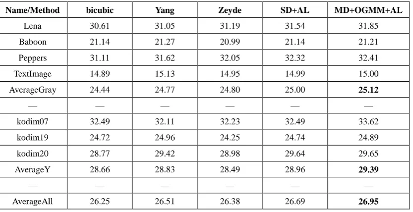
feature extraction
image blocking
i nt er pol at i on
Il I
Calculating the sparse representation and reconstruction error of each Dl
{
p
lk}
ˆIh
I
r min k lq
min rD
{
p
rk}
feature extraction
image blocking
i nt er pol at i on i nt er pol at i on
Il Il
II
Calculating the sparse representation and reconstruction error of each Dl
{
p
lk}
ˆIh ˆIh
I
r min k lq
min rD
min k lq
min rD
[image:3.595.86.511.440.706.2]{
p
rk}
Similar to other learning based methods, low and high
resolution training images are produced artificially as follows:
ASH A
j j
l h
y y v (1)
Where j h
y is jth original image regarded as a high resolution image, H denotes a blurring operator, S denotes a down
sampling operator, A denotes an interpolation process, v is an
additive Gaussian white noise. After a series of operations, jth
low resolution image j l
y is generated accordingly.
2.1.2
Image Patch Classification based on
OGMM in Principal Subspace
Features for image patch classification
The edge features of low resolution patch are chosen for
image patch classification. Each patch is filtered by 4
high-pass filtersf rr, 1, 2,3, 4, which are differential filters with first and second order, horizontal and vertical directions
respectively. From the four filtered images, four
corresponding patches which are size of n n and position atk, are extracted and concatenated into a complete feature vector k
l
p . Assume n=81, the dimension of k
l
p is 4*81=324. Obviously, if k l
p is directly adopted to classify patches or coupled dictionary learning and sparse
coding, the computation complexity will rather high. Hence,
the original feature space is first transformed into an
orthogonal space with K-L transform; then the principal
subspace is selected as the space in which image patch
classification is accomplished.
OGMM in principal subspace and image
patch classification
In brief, OGMM models the mixtures of Gaussian distribution
of the data in orthogonal space. Due to energy concentration
along the principal axis that features distribute, OGMM
achieves a more effective data distribution. Compared with
full-variance Gaussian mixture model, OGMM substantially
decreases the number of free parameters and thus reduces the
computational and storage cost of the related calculations. Its
formulation is defined as follows:
1
|
1
|
C
T
c c c c c c c
c
p x w
c
C
w O
x
(
, ,
,
,
, )
(
,
)
,
1 2 22
2
d c c c cx
x
/ /exp
(
)
, 11
C c cw
(2)Where x denotes the original feature vector and d is the dimension of it; C denotes the number of Gaussian mixture components, wc, φc and ∑c denotes the weights, mean vector
and diagonal covariance matrix of Gaussian components
respectively, is K-L orthogonal transform matrix. The
parameters of OGMM can be resolved by Expectation
Maximization (EM) algorithms. For the problem in this paper,
x is k l
p ; since k l
p must be compressed, the dimensionality of named principal subspace is in fact 324nl.The value of
l
n is determined by required preserved energy and super resolution scale. For instance in our work, the required
preserved energy is 99.9% and super resolution scale is 3,
l
n is about 48. EM algorithm is run to obtain ˆc andˆ ,c c 1 2, ,...,C , which are likelihood parameters of each image patch category. For each input
image patch feature k l
p , the likelihood T k| l c c p( p ˆ,ˆ ) of each category is calculated by equation (3) and the category
corresponding to the maximum likelihood is the patch
belonging to.
1
1 2 2 | 1 1 2 2 l T k l c c
T
T k T k
l c c l c
n c p p p p / / ˆ
( ˆ, )
ˆ
exp ˆ ˆ
ˆ
( )
(3)
2.1.3
Features for coupled dictionary learning
and alternative learning
Upon the classification results, coupled dictionary is learned
with alternative learning from the residual and low resolution
data of each category.
Features for coupled dictionary learning
A coupled dictionary contains two parts: residual part and low
resolution part. The former is learned from residual data, and
the latter is learned from low resolution data which is
compressed and projected adaptively upon its own
subspacec,c 1 2, ,C . Certainly, the two parts of coupled dictionary must be synchronized naming ‗coupled‘. It
is worth mentioning that why residual data other than high
International Journal of Computer Applications (0975 – 8887) Volume 41– No.10, March 2012
26 differences among subareas that contain more high frequency
components such as edges and texture patches. It is reasonable
that adopting residual data is capable of recovering more high
frequency lost by low resolution image.
Alternative Learning
Given residual data Prand low resolution data Pl, a coupled dictionary is learned by running the following alternative
learning.
Step 1:
The dictionary atom number is preset. The preset number of
data from Pror Plare selected randomly as an initialization of dictionary denoted asD(0)a . In following symbols, if Pb and ( )
Qn
a refer to low resolution data and dictionary, Pb and Dbrefer to high resolution data and dictionary and vice versa. Let n denotes iteration number and its initial value is 1.
Step 2:
NormalizeD(an1)
.
UtilizePaand normalized ( 1)
Dn a
, the sparse representation
( )
Qn
a is searched by orthogonal matching pursuit (OMP) algorithm [14].
2 ( 1)
E(Q) min Pa Dan Q
F
,s.t.
0
,
k
q
L
k
(4)( )
{Q }n arg min E(Q) a
Where L denotes the sparsity. The reason that the dictionary has to be normalized is OMP algorithm requires Euclidean
norm of atom to be 1.
Step 3:
UtilizePband pseudo-inverse of
( )
Qn
a ,D( )bn is obtained by MOD algorithm:
+
1( ) ( ) ( ) ( ) ( )
D
nP Q
nP Q
n TQ
nQ
n Tb b a b a a a
( )
D =Dr bn Or ( )
Dl Dbn (5)
Where ( )
Qn
a is a full-row rank matrix.
Exchange data and dictionary letting ( ) ( )
Dan Dbn
andPa Pb. In addition, n=n+1.
Step 4:
Execute step2 and step3 alternately until the preset iteration
number is reached. Finally,
ˆD
landD
lshould be normalized tobe
ˆD
randˆD
l.In equation (5), sparse representations of residual data and
low resolution data are used to get low resolution dictionary
or sparse representations of low resolution data and residual
data are used to get residual dictionary. The two computations
are executed alternatively for the purpose of synchronizing the
two dictionaries. That is to say, relying on identical sparse
representations, such a coupled dictionary could be employed
to approximate its own data with minimum or near minimum
representation errors. Step 2 and step 3 are performed
iteratively to further optimize the coupled dictionary. In
alternative learning, initial sparse representation (1)
Qa is also an extreme important, for it will affect the performance of
dictionary. Because the features of low resolution data rather
than residual data are compressed, residual data is selected to
initialize the dictionary D(0)r and
(1)
Qr is obtained correspondingly.
In addition, during reconstruction, the sparse representations
using ˆDl need to be compensated with atom length of
unnormalized dictionary Dl( ,d1dm) . The normalized
version of it is ˆD ( ,l dˆ1dˆm), dˆ1 dˆm 1. Thus,
2 2 1 1 2 1 1 2 1
ˆ
ˆ
ˆ
ˆ
P
D Q
P
(
,
,
)Q
ˆ
ˆ
ˆ
= P
( ,
,
)(
,
,
)Q
ˆ
ˆ ˆ
P
( ,
,
)Q
l l l m m
F F
l m m
F
l m
F
d
d
d
d
d
d
d
d
d
d
(6) 1 ˆ ˆQQ /( d ,, dm ),i1, 2,...,m (7)
Where m denotes the atom number, denotes the length of
each atom, each element of each column of ˆQis divided
by di ,i 1 2, ,m . In other words, ˆQ is obtained using ˆDlbut ˆQis required to estimate the residual data. Their relations are connected through equation (7).
Comparisons to other coupled dictionary
learning approaches
Other coupled dictionary learning approaches such as one
proposed by Yang [7]. He combined the features of low and
Lagrange Dual and Lasso algorithm. After the dictionary is
learned, it is separated into high and low resolution parts. The
dimension of joint feature is high, thus the computation
efficiency is relatively low. Zeyde [8] first learned the low
resolution dictionary using K-SVD algorithm, and then
learned the high resolution dictionary by MOD algorithm.
Apparently, the learning efficiency has been improved at cost
of declining reconstruction quality. We propose to learn the
coupled dictionary in alternative manner making them to be
synchronized. The convergence speed of alternative learning
is rapid such that only a few iterations are enough to get a
good result. Compared with Yang‘s and Zeyde‘s methods, the
proposed alternative learning has much higher efficiency and
excellent reconstruction quality has been demonstrated in the
experimental results.
2.2
Reconstruction Phase
The reconstruction phase composes four steps described
as follows:
1) Input image I is enlarged to be low resolution image Il
with scale s and bicubic interpolation algorithm.
2) Il is filtered with the same four high-pass filters as in
learning phase to produce a set of filtered
images{frIl r}1,2,3,4.Four n npatches are extracted
from the four filtered images in corresponding positions
denoted ask. The four patches are merged into a
feature vector k l
p , k=1, 2,…,N, where N refers to the total number of patches in Il.
3.1) k l
p is projected into each subspace c of each patch category to generate compressed feature
vector
c
k l
p ,c1, 2,...,C.The sparse representation of it
denoted as q
c
k
l is computed by ˆDlc of each coupled
dictionary and OMP algorithm.
3.2) Representation error 2
2
ˆ
Ec plkcD qlc klc is computed
for each category. Let
min
qk
l and ˆDrmindenote the sparse
representations and residual part of couple dictionary that
have gained the minimum representation errors. A
residual image patch ˆpkr corresponding to k l
p is thus
stimated with
min
ˆDr andqmin k
l . Notice that qmin k
l must be compensated as done in equation (7).
4) Position ˆk r
p in their original orders producing residual image Ir and overlapping exist between patches. The
pixel value of overlapped positions is an average of all
values at those positions. The sum of Il and Ir are adopted
as the reconstructed high resolution image ˆIh.
3.
EXPERIMENTAL RESULTS AND
ANALYSIS
The same training image set as the Yang‘s [7] is selected as
our training set. Altogether 80,000 patch pairs are sampled
randomly from the training set. To cope with color image,
RGB space is transformed into YCbCr space since Cb and Cr
channels contain much less high frequency. It means that only
Y channel is super-resolved and Cb-Cr channels are enlarged
with simple bicubic interpolation algorithms.
3.1
Objective Evaluation
Four grayscale images and three color images in Kodak's true
color image suite are chosen as test images. The up sample
scale is 3, and the objective evaluation criterion is peak
signal-to-noise ratio (PSNR, in dB).
The compared methods are bicubic interpolation, Yang‘s[7],
Zeyde‘s[8], single coupled dictionary with alternative
learning(SD+AL), multi-groups of coupled dictionary with
GMM and alternative learning (MD+OGMM+AL)
respectively shown in Table. 1. In the four dictionary-based
methods, the number of atom of each dictionary is all set
1024.
The boldface in table 1 shows that the method
MD+OGMM+AL has obtained the highest PSNR on average
level.
3.2
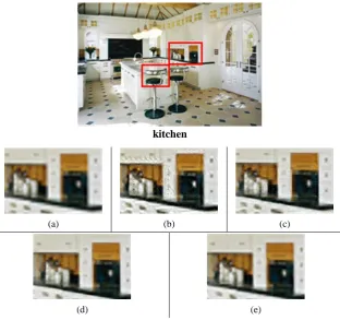
Subjective Evaluation
To compare super resolution reconstruction result from
subjective evaluation given by human visual system, we select
two color images named ―kitchen‖ and ―boat‖ with up sample
scale 3. The super resolution results of several regions
illustrated by red rectangles are emphasized in Fig 4, Fig 5,
Fig 6 and Fig 7 respectively. All the demonstrated regions are
their actual sizes.
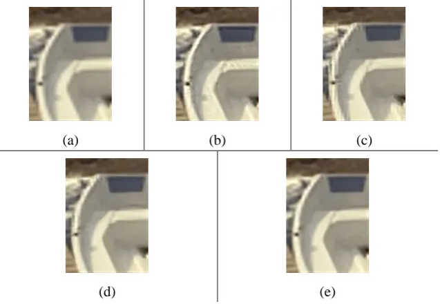
International Journal of Computer Applications (0975 – 8887) Volume 41– No.10, March 2012
28 has good sharpness around salient edges but pseudo-edges and
noise in local areas brought by reconstruction is also obvious.
The same artifacts have happened in Zeyde‘s method. For
(SD+AL) method, the reconstruction quality has been
improved to certain degree. From the comparison of Fig 6 and
Fig 7, (MD+OGMM+AL) is advantage over (SD+AL)
because the edges reconstructed by the former look more
natural and the sharpness is still preserved. Compared with
other methods, the super resolution image reconstructed by
the proposed multi-groups of dictionary has an appropriate
visual quality since its whole noise is the lowest and the
reconstructed edges demonstrate a good balance between
noise and sharpness. To sum up, a best reconstruction has
[image:7.595.120.475.190.369.2]been obtained by the proposed approach.
[image:7.595.92.509.415.629.2]Fig 3: Seven test images including four grayscale images and three color images
Table 1. Comparison of several super resolution methods in terms of PSNR
Name/Method bicubic Yang Zeyde SD+AL MD+OGMM+AL
Lena 30.61 31.05 31.19 31.54 31.85
Baboon 21.14 21.27 20.99 21.14 21.21
Peppers 31.11 31.62 32.05 32.32 32.41
TextImage 14.89 15.13 14.95 14.99 15.00
AverageGray 24.44 24.77 24.80 25.00 25.12
— — — — — —
kodim07 32.49 32.11 32.23 32.49 33.62
kodim19 24.72 24.96 24.25 24.74 24.89
kodim20 28.77 29.42 28.98 29.64 29.65
AverageY 28.66 28.83 28.49 28.96 29.39
— — — — — —
kitchen
(a) (b) (c)
[image:8.595.142.455.78.371.2](d) (e)
Fig 4: The results of different methods. (a) bicubic (b) Yang et al. (c) Zeyde et al. (d) SD+AL (e) MD+OGMM+AL
(a) (b) (c)
(d) (e)
[image:8.595.139.460.401.556.2]International Journal of Computer Applications (0975 – 8887) Volume 41– No.10, March 2012
30
boat
(a)
(b)
(c)
[image:9.595.143.458.76.434.2](d)
(e)
Fig 6: The results of different methods. (a) bicubic (b) Yang et al. (c) Zeyde et al. (d) SD+AL (e) MD+OGMM+AL
(a)
(b)
(c)
(d)
(e)
Fig 7: The results of different methods. (a) bicubic (b) Yang et al. (c) Zeyde et al. (d) SD+AL (e) MD+OGMM+AL
4.
CONCLUSIONS
Multi-groups of coupled dictionary and its alternative learning
are proposed in this paper. In learning phase, OGMM is
adopted to classify image patches in principal subspace of the
low resolution features. Then, joint features composed of
[image:9.595.140.459.463.683.2]respective category space are learned by alternative learning
to produce a coupled dictionary for each image patch category.
In reconstruction phase, low resolution feature of each input
image patch is first attempted to be reconstructed by using
low resolution part of couple dictionary. Next, the dictionary
that has gained least reconstruction errors is used to estimate
the residual patch. Finally, the residual image and low
resolution image are combined to generate a high resolution
image.
Multi-redundant dictionaries scheme is also applicable to
image self-learning. The reason of choosing an external image
set is as follows: 1) diversify the patch types for dictionary
learning and increase the quantity of learning data; 2) prevent
over-fitting due to the insufficient data caused by a too small
input image. It is well known that over-fitting will deteriorate
the performance of dictionary.3) the dictionary learned from a
specific image is only proper for itself; hence dictionary needs
to be relearn for each new image. Instead, general dictionary
learned from an outer image set could be used to reconstruct
arbitrary image without relearn. Further research maybe the
adaptive strategy: online modify the general dictionary
adaptively to a specific image so as to reach a good
efficiency-effectiveness tradeoff.
In fact, learning-based super-resolution reconstruction is a
highly open problem. It includes image patch feature
extraction, the feature compression, the atom number and
learning iteration number for dictionary learning and etc.
Currently, these issues are usually solved empirically and lack
of theoretical analysis. In the proposed scheme, the more
advanced image patch category model and reconstruction
scheme are both worthy of further studying topics.
5.
REFERENCES
[1] W. Freeman, T. Jones, E. Pasztor, "Example-based
super-resolution", IEEE Computer Graphics and
Applications, 22(2), pp. 56-65, 2002.
[2] H. Chang, Y. Yeung, Y. Xiong, "Super-resolution
through neighbor embedding", IEEE Conference on
Computer Vision and Pattern Recognition, vol. 1, pp.
275-282, 2004.
[3] T. Chan, J. Zhang, "Improved super-resolution through
residual neighbor embedding", Journal of Guangxi
Normal University, 24(4), pp. 211-214, 2006.
[4] T. Chan, J. Zhang, J. Pu, "Neighbor embedding based
super-resolution algorithm through edge detection and
feature selection", Pattern Recognition Letters, 30(5), pp.
494-502, 2009.
[5] K. Ni, T. Nguyen, "Image super-resolution using support
vector regression", IEEE Transactions on Image
Processing, 16(6), pp. 1596-1610, 2007.
[6] J. Yang, J. Wright, et al., "Image super-resolution as
sparse representation of raw image patches", IEEE
Conference on Computer Vision and Pattern Recognition,
pp. 1-8, 2008.
[7] J. Yang, J. Wright, T. Huang, Y. Ma, "Image
super-resolution via sparse representation", IEEE
Transactions on Image Processing, 19(11), pp.
2861-2873, 2010.
[8] R. Zeyde, M. Elad, M. Protter, "On single image scale-up
using sparse-representations", Curves & Surfaces,
Avignon-France, June 24-30, 2010.
[9] M. Aharon, M. Elad, A. Bruckstein, "The K-SVD: An
algorithm for designing of over-complete dictionaries for
sparse representations", IEEE Transactions on Signal
Processing, 54(11), pp. 4311-4322, 2006.
[10]K. Engan, S. Aase, "Method of optimal directions for
frame design", IEEE International Conference on
Acoustics, Speech and Signal Processing, vol. 5, pp.
2443-2446, 1999.
[11]M. Yang, C. Chu, Y. Wang, "Learning Sparse Image
Representation with Support Vector Regression for
Single-Image Super-Resolution", IEEE International
Conference on Image Processing, pp. 1973-1976, 2010.
[12] R. Zhang, X. Ding, "Offline handwritten numeral
recognition using orthogonal Gaussian mixture model", In
Proc. IEEE Int. Conf. on Image Processing, pp.
1126-1129, 2001.
[13]Zhang Xuegong, The nature of the Statistical Learning
Theory, Beijing: Tsinghua University Press, 2000.
[14]G. Davis, S. Mallat, Z. Zhang, "Adaptive time-frequency
decompositions", SPIE Journal of Optical Engineering,