Evolution of social norms with heterogeneous preferences: A general model and an application to the academic review process

Munich Personal RePEc Archive

Evolution of social norms with

heterogeneous preferences: A general

model and an application to the

academic review process

Azar, Ofer H.

Ben-Gurion University of the Negev

2002

Online at

https://mpra.ub.uni-muenchen.de/4482/

This is an early version of an article that is forthcoming in the Journal of Economic Behavior & Organization.The final version of this article is available at

http://dx.doi.org/10.1016/j.jebo.2006.03.006

Evolution of social norms with heterogeneous preferences:

A general model and an application to the academic review process

Ofer H. Azar

The article presents a model of social norm evolution, which suggests how the increase in

optimal and actual first response times (FRT) of economics journals can be related. When the

optimal FRT and the norm about how much time refereeing should take increase, it seems that

the existence of a norm increases the average refereeing time. The model suggests the surprising

result that this is not necessarily true. I also discuss applications of the model in other contexts,

differences in the optimal FRT between disciplines, the effects of the FRT on the tenure process,

and strategic behavior of referees.

JEL codes: Z13, L82, A14, I23, A10

Keywords: social norms; evolution; first response times; refereeing; academic publishing;

turnaround times; journals; review process.

1 _{Ofer H. Azar, Department of Business Administration, School of Management, Ben-Gurion University of the}

1.

Introduction

Academic publishing has received attention is several articles in recent years. A few

studies considered the pricing of academic journals (e.g. Bergstrom, 2001 and McCabe, 2002),

while others focused on various aspects of the review process, for example payment to referees

(Engers and Gans, 1998; Chang and Lai, 2001), the value-added from the review process

(Laband, 1990), and the increase in the number and the extent of revisions requested prior to

publication, which also increases the submit-accept time (Ellison, 2002a; 2002b). This trend is an

acknowledgement that research on the academic review process is not only interesting, but is

also very important, because knowing more about the process and understanding it better may

suggest how it can be improved, enhancing the productivity of economists and scholars in other

disciplines.

One of the most criticized aspects of the review process is the long delay in publication it

creates. The most important part of the editorial delay is the first response time (the time from

submission to first editorial decision, henceforth FRT): while most articles go through rounds of

revisions and the delay from acceptance to publication only in the journal that publishes the

article, the FRT is imposed on the article also in any journal that rejects it. Azar (2004a), for

example, estimates that the average article is submitted (and therefore suffers from the FRT) 3-6

times prior to publication.

A recent article (Azar, 2004b) suggests that the FRT of economics journals increased

from about 2 months 40 years ago to 3-6 months today. Interestingly, Azar argues that the

optimal FRT has also increased during this period. He explains that the optimal FRT is not zero,

because the delay caused by the FRT deters submissions of mediocre papers to good journals,

editors’ time).2 The optimal FRT is determined according to the trade-off between reducing the

review process costs and disseminating new research quickly. 3 Azar claims that because new

research today is often available as a working paper on the Internet even before publication in a

journal, it became less important from a social perspective to publish new research quickly in

journals. Moreover, because papers today are longer and more mathematical than in the past,

refereeing them is more costly, and therefore it became more important to deter frivolous

submissions. Azar explains that these two changes have increased the optimal FRT.

The fact that both the actual and the optimal FRT increased during the same period raises

several interesting questions. Did referees or editors think (consciously or not) about the optimal

FRT, and therefore the actual FRT increased together with the optimal FRT? What if some

referees do not care about the optimal FRT – are they also slower today than 40 years ago? If

referees follow a social norm in deciding how quickly to referee a paper, will this increase social

welfare or not? I address these questions and some other related questions using a model in

which referees care about several different things: the optimal FRT, the social norm about how

quickly a referee should respond, and their own personal preferences. I allow for heterogeneity

among referees in several dimensions and I analyze how the social norm evolves over time, in

particular when there is also an external change in the environment (e.g. an increase in the

optimal FRT). The model suggests the surprising result that even when the social norm changes

in a welfare-improving way, its existence may reduce welfare.

2 _{Azar (2006), however, offers a few ideas how the FRT can be shortened without increasing the costs of the review}

process.

While the discussion focuses on the review process, the model is more general and can be

applied to other contexts as well, thus contributing to the literature on the evolution of social

norms (see for example Sethi (1996) for an evolutionary model of social norms, Sethi and

Somanathan (1996) for an evolutionary model in the context of common property resource use,

and Azar (2004c) for a model which is applied to analysis of the tipping norm). I discuss briefly

two examples of other norms that can be analyzed using the model: workplace norms, and norms

of proper dress.

The rest of the article is organized as follows: Section 2 discusses potential reasons for

the increase in the FRT over the years. Section 3 presents a model of the evolution of social

norms applied to the refereeing context. The model is applicable to a broad range of social

norms; Section 4 discusses briefly two examples. Section 5 discusses three additional questions

regarding the FRT, and Section 6 concludes.

2.

The Slowdown in First Response Times of Economics Journals

Azar (2004b) suggests that the FRT grew from about 2 months circa 1960 to about 3-6

months today. What has changed over the last 40 years that could increase the FRT so much?

Technology obviously advanced significantly, but should have the opposite effect – to shorten

the FRT. With the software that exists today, it is easier to detect papers that spend too much

time in the referee’s hands. E-mail and faxes can be used for certain tasks and are faster than

mail. Electronic submissions were adopted by various journals and allow to eliminate the mailing

delays.

Ellison (2002a) documents an increase in the submit-accept time of economics journals

papers becoming longer and more complex). His empirical analysis, however, leads him to

conclude (p. 989), “What I find most striking in the data is how hard it seems to be to find

substantial differences between the economics profession now and the economics profession in

1970. The profession is not much larger. It does not appear to be much more democratic. I

cannot find the increasing specialization that I would have expected if economic research were

really much harder and more complex than it was 30 years ago.” Consequently, these issues also

do not seem to be the reason for the slowdown in the FRT.

Papers have become longer over the last few decades (see Ellison, 2002a; 2002b), and

this may increase the time needed to referee a paper. But refereeing most papers requires only a

few hours. Hamermesh (1994), for example, suggests that it takes six hours to referee an average

paper. The Canadian Journal of Economics provides advice to referees in which it states “The

amount of time taken with a paper can vary enormously – anything from a couple of hours to a

couple of days of full-time effort. A typical report should probably take 3 or 4 hours.”4 Assume

that today it takes on average five hours to referee a paper. No matter how little time it took to

referee a paper forty years ago, a few more hours required for the task today cannot justify an

increase of about three months in the FRT.

The FRT consists of the time it takes the editor to choose referees, the mailing time to

and from the referees, the time it takes the referees to write the reports, and the time it takes the

editor to make a decision based on these reports. The main component of the long FRT today is

the time the paper spends in the hands of referees. But it takes many referees a few months to

write a report not because they ponder about the importance of the paper for several months, but

because the paper waits a long time unread. In Franklin Fisher’s words, “Such a paper is delayed

not because a referee is taking three months to decide on it but because it is sitting in a pile on

his or her desk” (Shepherd, 1995, p. 103). Why do referees leave papers in the pile for more time

today than in the past? I suggest two reasons: because the social norm of how much time it

should take to referee a paper has increased, and because the optimal FRT is longer today.

The explanation why the optimal FRT has increased over the years was briefly discussed

in the introduction and appears in more detail in Azar (2004b). We might wonder how the

optimal FRT translates into referees’ behavior. Does it require that referees will compute the

optimal FRT or think about it explicitly? The answer is no, just as people might behave as if they

are utility maximizers even without actually solving a utility maximization problem. For

example, one of the two changes that increased the optimal FRT is the higher availability of

working papers today. Even without thinking explicitly about the optimal FRT, referees in the

past might have felt very guilty when it took them a long time to write their referee report

because they knew they were delaying the dissemination of this new research. Today, referees

know that the paper is probably already available on the Internet, and therefore they might feel

less guilty when delaying the review process.

Why are social norms related to the refereeing time (the time the paper spends in the

referee’s hands)? The refereeing time can be thought of as a social norm because when referees

contemplate how quickly they should send their report, they consider, directly and indirectly,

how quickly others write referee reports.5 That is, the refereeing time is affected by the norm

5 _{The indirect effect is that the editor’s expectations from the referee (and a major expectation deals with how}

quickly the report should be returned) are based on the behavior of other referees. Meeting the editor’s expectations

is important to referees for several reasons. First, the referee might feel irresponsible and uncomfortable when he is

about how much time it takes to referee a paper.6 Most referees today do not feel especially

embarrassed or guilty to send reports after three months, knowing that this is the time it takes

many other referees as well. But a few decades ago, when most referees responded within a few

weeks, it probably was much more embarrassing to send referee reports only after three months.

Comparison to other referees works also in the other direction: some referees may not want to be

faster than others, to avoid receiving too many refereeing requests (see Thomson, 2001, p. 116).

Obviously, if referees change their behavior because the optimal FRT has changed, this

also affects the social norm about how much time refereeing should take. The change in the

norm further affects referees’ behavior, so the norm changes again and so on. In what follows, I

introduce a dynamic model that describes the evolution of the social norm about refereeing time

and analyzes how the behavior of referees and the norm change when there are changes in the

environment (e.g. an increase in the optimal FRT).

when the referee is up for tenure or promotion Third, the treatment of the referee when he submits articles to the

journal may be affected by the editor’s opinion of him. Bad papers will be rejected anyway, but the decision about

marginal papers may be influenced (consciously or not) by the editor’s opinion of the author. Not only the editorial

decision, but also the choice of referees, may be affected by the reputation of the author as a referee. The Journal of

Finance even announced that the latter has been the journal’s policy: “We record both the time the reviewer took

and the quality of the review. The quality of the author as a reviewer is a strong influence on our decision of to

whom we will send the manuscript. Once again, the best way to ensure a good review is to be a good reviewer when

called upon” (Elton and Gruber, 1987).

6 _{See also Ellison (2002a, p. 984), who writes: “I use the term “social norms” to refer to the idea that the publication}

process may be fairly arbitrary: editors and referees could simply be doing what conventions dictate one does with

3.

The Evolution of the Social Norm of Refereeing Time

Let us think about a referee who receives a paper to referee, puts it aside for some time,

and then reads it and writes the report. The factors that affect the refereeing time chosen by the

referee (denoted by r) can be divided to three: the social norm about how long it should take to

referee a paper, the optimal delay (denoted by D*), and all other factors.7 These other factors

include how busy the referee is, how much he tends to procrastinate, whether the paper interests

him, and so on; I denote the delay that the referee would choose if these were the only factors by

v (“various factors”), which may differ across referees. The preferred refereeing time from the

referee’s perspective (ignoring the social norm for the moment) is denoted by p, and is equal to a

weighted average between D* and v:

( 1 ) p = wD* + (1 − w)v.

The weight given to the optimal delay, w ∈ [0, 1], may be different across referees. Referees

who do not care at all about the optimal delay correspond to w = 0, for example. Notice that

while p, w and v are potentially different across referees, D* is the same for everyone.8

The relative importance of the social norm for each referee is measured by m, where 0 ≤

m < 1. The values of m, p, v, and w represent the referee’s personality and concerns and are

exogenous. The referee only chooses the refereeing delay, r. The desire of the referee to choose a

7 _{The optimal delay is the optimal refereeing time (from a social perspective). It equals the optimal FRT minus the}

time that the paper spends in the editor’s hands and in the mail to and from the referee. A longer optimal FRT

therefore increases also the optimal delay.

8 _{The notation also makes it easy to remember which variables are potentially heterogeneous: capital letters denote}

refereeing delay that is close to p on one hand, but also close to the norm in period t (denoted by

Nt) on the other hand, is expresses in the following utility function:

( 2 ) u(r; p, m, Nt) = − m(r − Nt)2− (1 − m)(r − p)2.

Taking the first-order condition of the utility maximization problem and rearranging

suggests that the optimal choice of r in period t (denoted rt) is given by the weighted average of p

and Nt:

( 3 ) rt = mNt + (1 − m)p = mNt + (1 − m)[wD* + (1 − w)v].

The social norm in period 0 is arbitrarily determined and denoted as N0, and afterwards it

evolves as follows: the norm in period t ≥ 1 is equal to a weighted average of the norm in the

previous period and the average refereeing delay in the previous period. That is,

( 4 ) Nt = zNt−1 + (1 − z)E(rt−1),

where E(rt−1) is the average of r (over all the referees) in period t−1 and z is a parameter

satisfying 0 ≤ z < 1. To examine how changes in the environment affect the long-run social

norm, we should find the equilibrium level of the norm. One possible definition for the

equilibrium level of the norm is the level to which the norm converges. An alternative definition

is the value N such that if Nt = N then Nt+1 = N. The following proposition suggests that the two

definitions are equivalent, and also computes the equilibrium level of the norm, which I refer to

also as the “stable norm” or N∞.

Proposition 1: The social norm converges to N∞ ≡ E[(1 − m)p] / [1 − E(m)]= E(p) −

cov(m, p)/[1 − E(m)], where cov (m, p) is the covariance of m and p over all the referees, and

norm is equal to N∞ it does not change anymore as long as the environment (the distribution and

preferences of referees, the optimal delay, etc.) remains the same.

Proof: Using equations ( 3 ) and ( 4 ) we get Nt = zNt−1 + (1 − z)E(rt−1) = zNt−1 + (1 −

z)E[mNt−1 + (1 − m)p] = Nt−1[z + (1 − z)E(m)] + (1 − z)E[(1 − m)p]. Since this is true for all t, as

long as t is large enough, we can express Nt−1 as a function of Nt−2, and then Nt−2 as a function of

Nt−3 and so on. For notational convenience, let us define first x = z + (1 − z)E(m) and y = (1 −

z)E[(1 − m)p]. It then follows that Nt = xNt−1 + y = x(xNt−2 + y) + y = x[x(xNt−3 + y) + y] + y =

… Continuing in this fashion establishes that for any integer k such that k ≤ t we have:

( 5 ) Nt = xkNt−k + y(1 + x + x2 + … xk−1).

To proceed, notice that x can be thought of as a weighted average of 1 and E(m), with a

strictly positive weight given to E(m) (a weight of 1−z, and recall that 0 ≤ z < 1). Since m ∈ [0,

1), it follows that E(m) ∈ [0, 1) and therefore x ∈ [0, 1). As t →∞, the equation is true for values

of k that approach infinity, implying that xk → 0 and that the expression in parentheses

approaches 1/(1 − x). Using these observations and substituting for x and y we then obtain:

lim t→∞ Nt≡ N∞ = y / (1 − x) = (1 − z)E[(1 − m)p] / [1 − z − (1 − z)E(m)] = (1 − z)E[(1 − m)p] /

(1 − z)[1 − E(m)] = E[(1 − m)p] / [1 − E(m)]. Rearranging, substituting E(mp) = cov (m, p) +

E(m)E(p), and then simplifying, shows that this expression is equal to E(p) − cov(m, p)/[1 −

E(m)]. To see that if Nt = N∞ then Nt+1 = N∞ it is again simpler to use the definitions of x and y.

Notice that Nt+1 = xNt + y = xN∞ + y = xy/(1 − x) + y = [xy/(1 − x)] + [y(1−x)/(1−x)] = y[x + (1

− x)]/(1 − x) = y/(1 − x) = N∞. Q.E.D.

Proposition 1 suggests that we have a well-defined notion of equilibrium in the model,

norm; it does affect the speed of convergence, however. The result that the stable norm equals

E(p) − cov(m, p)/[1 − E(m)] has an interesting intuition. In the absence of a social norm, each

referee chooses a delay equal to his p and therefore the average refereeing time is equal to E(p).

With a social norm, the average refereeing time (which is also the norm) is higher than E(p) if

and only if cov(m, p) < 0 (since E(m) < 1). The intuition why this holds is that people with a low

m put a little weight on the norm and a high weight on their own preference (p). Consequently,

cov (m, p) < 0 implies that those with a high p care less about the norm than those with a low p;

as a result, those with a high p affect the others more than the others affect them (through the

social norm). Therefore the average refereeing time is higher than in the absence of a social norm

– higher than E(p). The intuition why cov (m, p) > 0 implies that N∞ < E(p) follows a similar

argument.

A natural question is whether the stable norm is higher, lower, or equal to the optimal

delay. The following proposition suggests a simple expression that determines whether the stable

norm is higher than the optimal delay:

Proposition 2: The value of (N∞− D*) is equal to E[(1 − m)(1 − w)(v − D*)]/[1 − E(m)]. It

follows that the sign of (N∞− D*) is the same as the sign of E[(1 − m)(1 − w)(v − D*)].

Proof: Using Proposition 1 and substituting for p from equation ( 1 ) we get that N∞− D*

= E{(1 − m)[v(1 − w) + D*w]}/[1 − E(m)] − D*. Rearranging this expression then yields {E[(1 −

m)v(1 − w)] + D*[E(w) − E(mw) − 1 + E(m)]}/[1 − E(m)], which after further simplification

becomes E[(1 − m)(1 − w)(v − D*)]/[1 − E(m)]. Since m ∈ [0, 1), the denominator is strictly

Proposition 2 shows that E(v) = D* does not guarantee that the stable norm is equal to the

optimal delay. It also suggests that higher values of v make it more likely that the stable norm is

higher than the optimal delay, and vice versa. In particular, if v ≥ D* for all referees, then N∞ ≥

D*, and vice versa. In addition, (N∞− D*) is strictly increasing in the value of v of any referee for

whom w < 1. This implies that from a social-welfare perspective, if the stable norm is higher

than the optimal delay, we would like to reduce the values of v of the referees. There are various

ways to reduce the value of v, for example to pay referees for a report that is written in a short

time. It is worth pointing out that

An interesting question to ask is how a change in the environment affects the stable norm.

In particular, what is the effect of an increase in the optimal delay on the social norm? How does

it affect individual referees? The following proposition answers these questions.

Proposition 3: (i) A change in D* from D*0 to D*1 changes the stable norm by (D*1 −

D*0)E[(1 − m)w] / [1 − E(m)]. This implies that if no referee cares about the optimal delay (w =

0 for all referees), then a change in D* does not affect the stable norm. Otherwise, the stable

norm changes in the same direction as the change in D*. If w < 1 for at least one referee, then

the change in the norm is smaller than the change in D*.

(ii) Assume that at least some referees care about the optimal delay. Then, every referee

will change his choice of r in the direction of the change in D*, except for referees who do not

care about the norm (m = 0) and also do not care about the optimal delay (w = 0), who do not

change their choice of r.

Proof: (i) We want to compare the stable norm before and after the change in D*,

assuming that all other parameters (m, v, and w) are unchanged (p is changed because it is a

and N∞1, respectively. Similarly, denote the values of p before and after the change as p0 and p1

(each referee may have different values of p0 and p1, however). Using Proposition 1 and equation

( 1 ) and rearranging we get: N∞1− N∞0 = E[(1 − m)(p1− p0)] / [1 − E(m)] = E[(1 − m)w(D*1−

D*0)] / [1 − E(m)] = (D*1− D*0)E[(1 − m)w] / [1 − E(m)]. Since m ∈ [0, 1), the denominator is

strictly positive, and so is the term (1 − m) in the expectation in the numerator. If w = 0 for all

referees, the numerator is equal to zero, implying that the stable norm does not change. If w > 0

for at least one referee, however, the numerator has the same sign as (D*1 − D*0), implying that

the norm changes in the same direction as the change in the optimal delay. To see that the change

in the norm is smaller than the change in D*, notice that since (1 − m) is strictly positive and w is

smaller than 1 for at least one referee, it follows that E[(1 − m)w] < E[(1 − m)*1] = 1 − E(m) and

the change in the stable norm is strictly smaller than the change in D*.

(ii) Recall from equation ( 3 ) that rt = mNt + (1 − m)[wD* + (1 − w)v]. Denote the choice of r

with a stable norm before and after the change in D* as r∞0 and r∞1. It follows that r∞1 − r∞0 =

m(N∞1− N∞0) + (1 − m)w(D*1− D*0) = m(D*1− D*0)E[(1 − m)w] / [1 − E(m)] + (1 − m)w(D*1−

D*0) = (D*1− D*0){mE[(1 − m)w] / [1 − E(m)] + (1 − m)w}.9 Since the assumption in this part is

that some referees care about the optimal delay (w > 0), it follows that E[(1 − m)w] > 0. Since m

∈ [0, 1) and w ∈ [0, 1], it follows that (r∞1− r∞0) has the same sign as (D*1− D*0), unless both m

= 0 and w = 0 (in this latter case, r∞1− r∞0= 0). Q.E.D.

Part (i) of Proposition 3 suggests that it is sufficient that at least one referee cares about

the profession’s welfare (and therefore about the optimal delay) in order for the social norm to

9 _{Recall that m and w are the specific parameters of the individual referee, whereas E[(1 − m)w] and E(m) are the}

change in the direction of the optimal delay. Since the optimal delay increased in the last few

decades, Proposition 3 provides a potential explanation why the social norm, or the mean

refereeing time, increased as well.

In addition, since the social norm increases in the period following the change in the

optimal delay, referees further increase their delay, the norm increases even further and so on.

Despite this recurring increase in the norm, however, the proposition tells us that the overall

increase in the norm is still smaller than the change in the optimal delay (with w < 1 for at least

one referee). Part (ii) of Proposition 3 implies that even referees who do not care about the

optimal delay (w = 0) increased their refereeing time because of the change in the social norm,

except for the extreme case in which they do not care at all also about the norm.

It seems that the social norm is a mechanism that reinforces the tendency of referees to

change their behavior in the direction of the change in the optimal delay. For example, suppose

that the optimal delay increases. Referees change their preferences toward a higher delay (p

increases because D* increases). This implies that referees choose higher values of r; doing so

increases the norm, which further increases the values of r chosen by the referees and so on. It

seems that the existence of the social norm magnifies the increase in the average refereeing time

(which is by definition the stable norm). The following proposition suggests the surprising result

that this is not necessarily true.

Proposition 4: Assume that the optimal delay changed, and denote the change by ∆D*

(which is positive if D* increased and vice versa). Denote the change in the stable norm if

norm when referees care about the norm as ∆Nm>0 (the distribution of w remains the same).10 We

then have ∆Nm=0 − ∆Nm>0 = cov (m, w)∆D*/[1 − E(m)], implying that the sign of (∆Nm=0 −

∆Nm>0) is the same as the sign of [cov (m, w)∆D*], where cov (m, w) is computed when referees

care about the norm (when they do not the covariance is 0 since m = 0 for all referees).

Proof: Using Proposition 3 and substituting m = 0 and E(m) = 0 when referees do not

care about the norm, we get that ∆Nm=0 − ∆Nm>0 = ∆D*E(w) − ∆D*E[(1 − m)w]/[1 − E(m)] =

∆D*{E(w)[1 − E(m)] − E[(1 − m)w]}/[1 − E(m)] = ∆D*[E(mw) − E(w)E(m)] /[1 − E(m)] = cov

(m, w)∆D*/[1 − E(m)], where all the expressions involving m refer to the case in which referees

care about the norm (m = 0 was already substituted for the other case). The fact that E(m) ∈ [0,

1) completes the proof. Q.E.D.

Since the norm changes in the direction of ∆D* (see Proposition 3), Proposition 4

suggests the surprising result that when cov (m, w) > 0, the stable norm changes more when

referees do not care about the norm (whether ∆D*is positive or negative). The intuition for this

10 _{Some readers may find the term “the average delay in the long run when there is no social norm” more intuitive}

than “the stable norm if referees do not care about the norm.” The two expressions, however, are equivalent, since

the stable norm is by definition the average delay (in the long run) and “no social norm” is equivalent to the case in

which there is a norm but m = 0 for all referees. The latter equivalency is intuitive, and can also be seen formally: if

no social norm exists, each referee chooses a delay equal to his value of p (to see this, maximize the utility function

in ( 2 ) after eliminating the first term, which includes the norm), and the average delay is E(p). If we use the

framework developed so far and substitute m = 0 and E(m) = 0 in Proposition 1, we also get N∞ = E(p). I find it

more convenient to stick to the established framework and substitute m = 0, and therefore I use the somewhat

result is as follows (assume, without loss of generality, that the optimal delay increased; the same

idea is true when it decreased): when referees care about the norm, the norm indeed increases the

delay of those who do not care much about the optimal delay. At the same time, however, since

the norm is affected by those who do not care about the optimal delay, the norm reduces the

delay of those who care about the optimal delay. These two effects of the norm act in opposite

direction on the average delay, and which one dominates depends on cov (m, w). When cov (m,

w) > 0, it implies that generally, those who care a lot about the optimal delay (high value of w)

also care more about the norm (high value of m). Since they care more about the norm, they are

more affected by the others than they affect the others, leading the average delay to increase less

than if no one cared about the norm.

An interesting question is whether the existence of the social norm improves social

welfare. Non-existence of the norm is equivalent to assuming m = 0 for all referees; the stable

norm is useful because it equals the average delay, but the norm has no effect on the behavior of

individual referees (see the last footnote). Let the subscripts m>0 and m=0 denote the cases

where referees care or do not care about the norm, respectively (as in Proposition 4), and denote

the absolute value of (v − D*) by |v − D*|. The next proposition describes the effect of the norm

on social welfare (denoted by W):

Proposition 5: Assume that W is strictly concave in the delay and that either W is

symmetric in d, or that (N∞− D*)m>0 and (N∞− D*)m=0 have the same sign. Welfare is then higher

when referees care about the social norm if and only if cov [m, (1 − w)|v − D*|] > 0; welfare is

lower when referees care about the social norm if and only if cov [m, (1 − w)|v − D*|] < 0.

Proof: Since W is concave in the delay, a higher deviation (in absolute value) of N∞ from

same direction. If at least one of these conditions is met, then welfare is higher when referees

care about the social norm if and only if |N∞ − D*|m=0 − |N∞ − D*|m>0 > 0 (and welfare is lower

when referees care about the social norm when this expression is negative). Using Proposition 2,

substituting m = 0 in the case when referees do not care about the norm and rearranging yields

that |N∞ − D*|m=0 − |N∞− D*|m>0 = E[(1 − w)|v − D*|] − E[(1 − m)(1 − w)|v − D*|]/[1 − E(m)] =

{[1 − E(m)]E[(1 − w)|v − D*|] − E[(1 − m)(1 − w)|v − D*|]}/[1 − E(m)] = {E[m(1 − w)|v − D*|] −

E(m)E[(1 − w)|v − D*|]}/[1 − E(m)] = cov [m, (1 − w)|v − D*|]/[1 − E(m)]. The proposition then

follows immediately from 0 ≤ E(m) < 1. Q.E.D.

Proposition 5 suggests that the social norm can increase or decrease social welfare,

depending on the characteristics of referees (the distribution of m, w, and v). Other things being

equal, welfare is likely to be improved by the social norm when relatively high values of m are

associated with relatively low values of w (relative to the distributions of m and w). In particular,

if v is the same for all referees (and different from D*), the condition for the social norm to be

welfare improving becomes cov (m, w) < 0. The intuition is similar to the one discussed before.

Referees improve welfare more the closer their personal preference is to the optimal delay,

which happens when they have high values of w. The social norm creates two opposite effects:

the “bad” referees (whose w-value is low and therefore their preferred delay is far from the

optimal delay) affect the “good” referees (high w-values) negatively, but the good referees affect

the bad referees positively. The positive effect dominates when the good referees are less

affected by the social norm than their bad colleagues. Since m measures the effect of the norm,

4.

Additional Applications of the Model

While the model is used here to discuss the review process, it has many other

applications. One example is that of workplace norms. Workers are often affected by the effort

level of other workers around them, either because it gives them an idea of what is considered

appropriate and they feel guilt if they are much lazier than their colleagues, or because of direct

peer pressure. Pressure can go either way: if workers receive a bonus that depends on the firm’s

profits, the pressure is to work hard. If workers are afraid that they will be measured in

comparison to the most productive workers (and especially if a quota or a pay-for-performance

scheme is determined according to the achievements of the best workers), the pressure is not to

work too hard.

The assumption that the social norm enters the utility function is therefore reasonable in

the context of the workplace. What about the rest of the model? Clearly, workers have additional

characteristics that determine how hard they want to work, and there is heterogeneity in these

characteristics. One alternative to apply the model is to think about the hard workers as those

who care more about the level of effort that is optimal for the firm. Naturally, this level (D*) is

higher than the level implied by the worker’s various other reasons (v), implying that workers

who care more about what is optimal for the firm (higher w) have a personal preference for a

higher effort level (higher p). But we can also use a simplified version of the model, assuming

that no one cares about what is optimal for the firm (w = 0). It then follows that p = v, but since

the model allows v to vary across agents, we can still capture worker heterogeneity (in desired

effort) in our analysis.

Proposition 2 now suggests that the average effort level is lower than the optimal effort

the social norm increases the average effort level, thus increasing the firm’s profit. The intuition

is that cov (m, p) < 0 means that those who work harder (high p) are in general less affected by

the norm (low m). Consequently, the effect of the good workers on the bad workers is stronger

than the opposite effect. The opposite occurs when cov (m, p) > 0. One implication of the model

is that the firm should prefer a worker that is not affected by others if he is a hard worker by his

nature, but a worker who is affected by his colleagues if he is a relatively lazy worker.

Moreover, the insights of the model apply also when there is no optimal action at all. For

example, consider dressing norms, and suppose that there are two types of people: those who

prefer to dress elegantly, and those who prefer to dress simply (because it is cheaper or more

convenient, for example). Everyone, however, is also concerned by the norm and suffers some

disutility that increases as his deviation from the norm increases, as in the model (assume that

elegancy of dress is a continuous variable; the norm is the average choice of elegancy). By the

same analysis as in the model, if the elegancy lovers are concerned about the norm more than the

simplicity lovers, the norm will make the average clothes simpler than if no one cared about the

5.

Discussion

5.1. The Optimal First Response Time in Different Disciplines

There are several interesting questions about the optimal FRT and the evolution of the

refereeing delay that I want to address below.11 The first question is why in many other

disciplines the FRT is much shorter than in economics. As an example, let me take the case of

physics. While in economics the average FRT is a few months, in physics it is a few weeks.

Suppose that the optimal FRT in economics is indeed a few months, because the long FRT

prevents submissions of mediocre papers to good journals and therefore reduces the costs of the

review process (for further discussion of the optimal FRT in economics see Azar, 2005). Can we

infer that the FRT in physics is much shorter than optimal?

The answer is no. The disciplines are different in many important ways, and these

differences result in a different optimal FRT. One of the main determinants of the optimal FRT is

the social cost associated with delaying the publication of new research. This cost is lower today

than in the past because of the availability of working papers on the Internet. The cost was not

eliminated, however, because not all research is posted on the Internet, and because the

certification of quality that journals offer is important: the signal they provide allows readers to

save their scarce time for reading only the best research. This social cost is higher in disciplines

in which published research affects further research more rapidly (let us call these “immediate”

disciplines). If research today uses mostly findings from research conducted a few months ago,

11 _{I thank the Editor, J. Barkley Rosser, Jr., for suggesting these questions; I present here a short discussion of these}

questions, but the questions are important enough to justify a fuller treatment in separate articles and are therefore

then it is much more important to disseminate new research quickly than if research today is

based on previous research conducted 15 years ago. Is physics a more immediate discipline than

economics?

The answer is unambiguously yes. Journal Citation Reports (JCR) of Thomson ISI

records data on citations in various journals and disciplines. JCR includes 8 different

sub-disciplines of physics, which I aggregated by summing the number of citations, journals, and

articles, and averaging the immediacy index and the cited half-life index. Table 1 compares

economics and physics, based on the data in JCR of 2004.

Table 1: Characteristics of Economics and Physics

Total cites Number of

articles

Cites /

articles

Number of

journals

Immediacy

index

Cited

half-life

Economics 148,130 7,490 19.8 172 0.139 > 10.0

Physics 2,055,985 95,635 21.5 285 0.502 6.7

The two measures that indicate immediacy of a discipline are the immediacy index and

the cited half-life number. The immediacy index is the average number of times an article is

cited in the year it is published, and it indicates how quickly articles in the subject category are

cited. If in one discipline papers are cited much more (per article) than in another, this can also

increase its immediacy index, but we can see in the “Cites / articles” column that each article is

cited on average a similar number of times in both disciplines. Physics, however, has an

immediacy index which is about 3.6 times that of economics, indicating that physics is a much

Another measure that shows this is the cited life. JCR explains that “The cited

half-life for the category is the median age of its articles cited in the current JCR year. Half of the

citations to the category are to articles published within the cited half-life.” In economics the

median cited article was over 10 years old; in physics it was 6.7 years old.12 These two findings

suggest that in physics new research is used as the background for further research much more

quickly than in economics. Consequently, in physics the social cost of delaying publication of

new research is higher, and the optimal FRT is lower.

Another important determinant of the optimal FRT is the cost of the review process,

which is mostly the time of editors and referees involved in the process. I am aware of no hard

data on how much time a referee spends on a paper, but a reasonable conjecture is that a longer

paper requires more hours of work. Table 2 presents data about the average article length in

several top journals in economics and physics.

12 _{The highest category for cited half-life in JCR is “>10.0 years”, so an exact number is not available in economics,}

but the median is only slightly above 10 years, because the last 10 years account for 49.76% of the citations in

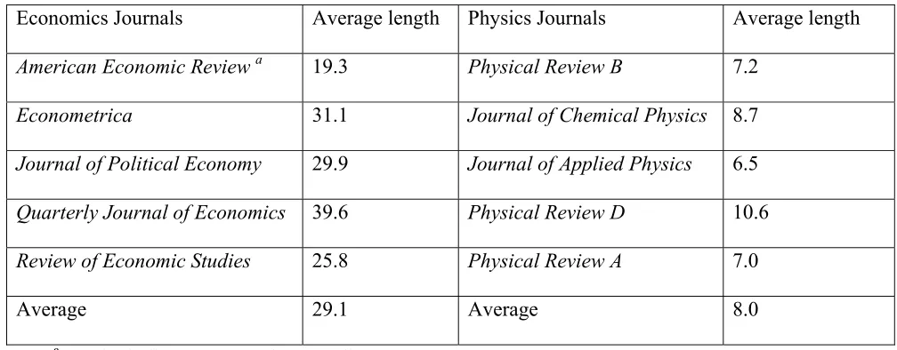
Table 2: Article Length in Top Journals in Economics and Physics

Economics Journals Average length Physics Journals Average length

American Economic Review a 19.3 Physical Review B 7.2

Econometrica 31.1 Journal of Chemical Physics 8.7

Journal of Political Economy 29.9 Journal of Applied Physics 6.5

Quarterly Journal of Economics 39.6 Physical Review D 10.6

Review of Economic Studies 25.8 Physical Review A 7.0

Average 29.1 Average 8.0

a

Not including Papers and Proceedings.

Because in economics papers are much longer than in physics, it means that the social

cost of a submission is higher in economics, because the referees are likely to need more time to

read the paper. As a result, it is much more important to deter frivolous submissions in

economics than in physics, once again resulting in a higher optimal FRT in economics.

Consequently, even if in economics the optimal FRT is a few months, it is possible that in

physics the optimal FRT is a few weeks.

5.2. First Response Times and Untenured Faculty

A second intriguing issue is the effect of the FRT on untenured professors and on the

tenure process in general. The common wisdom is that the people who get hurt the most from the

current long FRTs in economics are untenured faculty. They must obtain a certain number of

publications in order to get tenure, and the long delays in the publication process (especially the

FRT, which can delay the same paper several times, if the paper is rejected from a few journals

common wisdom and claim that getting tenure is not harder because of the long FRTs in

economics; nevertheless, I will explain why the long FRTs do have adverse effects on untenured

faculty and in the tenure process more generally.

The reason why long FRTs do not make it harder to get tenure is essentially that the

tenure decision is a tournament. The candidate to be tenured has to show that given the quality of

the institution he works at, his publication record is satisfactory. What determines how many

publications (and in which journals) are sufficient to be considered satisfactory? A comparison to

other young researchers at the institution and elsewhere does. So the tenure process is essentially

a competition among untenured faculty. The best ones get tenure at the best places, the ones with

slimmer publication records either get tenured in lower-ranked schools, or leave academia. In a

competition, if something makes the task harder for anyone, there might be winners and losers,

but it cannot be that everyone ends up in a lower rank than otherwise. What this means in our

context is that if FRTs were shorter and young faculty could get more publications by the time

they are up for tenure, the tenure committees would have required more publications in order to

get tenure. Consequently, the average untenured professor is not less likely to get tenure with

long FRTs than with shorter FRTs but higher expectations.

The long FRTs, however, do hurt untenured faculty somewhat; not in getting tenure, but

in putting them in a disadvantage compared to tenured faculty (in addition to the obvious

disadvantage…). Untenured faculty have little time to produce several publications, and because

of the high rejection rates of top journals, they should adopt an impatient submission strategy and

go down the list of journals (in terms of their quality) relatively quickly. It is a risky strategy for

untenured faculty to submit a paper to several top general journals before starting to submit it to

strategy is risky because the author can find himself without enough publications by the time of

his tenure decision (for a formal model that analyzes optimal submission strategy, see Azar,

2005).

Tenured faculty, on the other hand, have much less time pressure, and can therefore go

down the list of journals to which they submit more slowly. Because they can adopt a more

patient submission strategy and try more top journals before giving up and submitting to

lower-quality journals, tenured faculty have better chances to publish in top journals, given a constant

quality of the submitted paper. Thus, untenured faculty are at a disadvantage compared to

tenured faculty.

There is, however, a social cost related to the tenure process because of the long FRTs.

Publication records are shorter than they could be with shorter FRTs, and papers that could

already be published with shorter FRTs are still working papers. This makes it harder to evaluate

the quality of these working papers (if they were published, the identity of the journal that

published them would have provided an informative signal about their quality). This can result in

two things: first, it might require more effort from the tenure committee and from people who

write reference letters about the candidates for tenure. For example, they might have to read a

few of the candidate’s working papers in order to evaluate them, instead of observing which

journals published them (which could be the case with shorter FRTs). Second, less information

implies that the process becomes more prone to mistakes, in both directions: denying tenure to

people who are above the institution’s standards and vice versa.

The above discussion suggests that the optimal FRT is lower when considering its

implications on the tenure process than what it would be absent these implications. But it does

deterring submissions of mediocre papers to good journals and thus reducing the costs of the

refereeing system.

5.3. Selfish Strategic Behavior and the Evolution of the Refereeing Delay

A third interesting question is how the desire to avoid receiving too many refereeing

requests affects the evolution of the refereeing delay. If one wants to minimize the number of

refereeing requests he receives, being a slow referee can help him achieve this goal: editors will

learn of his tardiness and will be less inclined to send him additional requests to referee in the

future13; the referee will also have more papers waiting to be refereed on his desk, and will thus

be able to refuse to additional refereeing requests with the excuse that he already has too many

referee reports to write (assuming that referees use this excuse only when it is true). I believe,

however, that such strategic behavior is uncommon. After all, someone who wants to minimize

the effort he makes on refereeing activities can simply decline the refereeing requests he receives

rather than be slow in returning the report.

There are two main reasons that lead people to agree to refereeing requests despite the

effort required. One is that they are altruistic and they realize that the review process is a public

good to which one should contribute when asked to do so. The second reason is more selfish:

they want to retain good relations with the editor; he might be asked one day to write a letter of

reference about them, and he also can affect the outcome when they submit papers to this

journal.

13 _{An interesting anecdote is that the editors of the Economic Journal in the early 1970s report that any referee who}

took more than 2 months to return his report was dropped from the list of referees, unless there was a good reason

for the delay (Champernowne, Deane and Reddaway, 1973); today an economics journal with a similar policy is

If the referee agrees because he is altruistic, then he probability realizes that contributing

to the academic community requires not only writing referee reports, but also writing them in a

timely manner. If the referee agrees because he wants to retain good relations with the editor, he

also understands that being very slow will annoy the editor and can hurt him in the future. Those

for whom neither reason is important (they are neither altruistic nor do they value good relations

with the editor), should simply refuse to referee rather than be very slow. They will save

themselves a lot of effort, and even the author and the journal will be better off.

It might still be the case that because of such considerations of not being a referee who is

too good (and therefore receives many refereeing requests), people will be slower than

otherwise. There are two main ways to represent such behavior in the model, depending on what

assumptions we have regarding this behavior. If we assume that people will choose refereeing

delays very close to the norm so that they are not much faster than others, this can be captured by

a higher value of m than otherwise.14 If we assume, however, that people will be slower because

of strategic considerations regardless of the norm, this can be captured by a higher value of v. In

the latter case it is clear that this strategic behavior will lead to a longer norm of refereeing delay

(and a longer FRT). If the FRT is already longer than the optimal FRT even without strategic

behavior, it follows that this strategic behavior increases the difference between the optimal and

the actual FRT and thus reduces social welfare.

If the trade-off between avoiding too many refereeing requests and keeping good

relations with the editor (or altruistic motivations) is such that the optimal behavior is always to

be slightly slower than the norm, we can have a situation where everyone tries to be a little

14 _{Notice, however, that a higher value of m also implies that people who tend to choose a refereeing delay higher}

slower than the norm, this results in the norm becoming longer, people then choose a delay

slightly longer than the new norm, and so on. In this case the refereeing delay can become longer

and longer even without any increase in the optimal delay.

While such strategic behavior possibly contributed to the slowdown in the FRT since the

1960s, there are several reasons why it does not seem to be the major reason for the slowdown.

First, it requires that the optimal behavior for most people is to be slower than the norm,

something that is not obvious given that both altruistic motivations and retaining good relations

with the editor are reasons to be a fast referee. Second, why didn’t strategic behavior cause a

similar slowdown in refereeing in other disciplines, such as physics?

Finally, if this is a major reason for the slowdown, why did the slowdown start only in

the 1960s? Champernowne, Deane and Reddaway (1973), for example, report that between

January 1, 1971 and June 13, 1972, the Economic Journal obtained 286 referee reports, of which

158 were written in less than 3 weeks. Marshall (1959) sent questionnaires to editors of 30

economics journals, and received usable answers from 26 journals. Out of these 26 journals,

Marshall reports that “Twenty-three editors reported that they gave notification one way or the

other within 1 to 2 months, and only 2 editors reported a time-lag of as much as 4 months or

more.” If editors could make a decision in 1-2 months, including the time it takes to mail the

paper to and from the referees and the time it takes editors to choose referees and read their

reports, this means that referees were very quick, writing a report in less than a month.

Presumably, referees in the 1930s did not write reports much faster than the referees in the

1960s. It then requires an explanation, if referees have an incentive to be slower than the norm

and this is what caused the slowdown in the FRT, why did it start only in the 1960s or 1970s and

6.

Conclusion

The review process in economics is an important research topic since insights about it can

help us improve the process and increase the productivity of economists and other scholars.

Previous research suggested that the optimal and the actual FRT both increased over the last few

decades (Azar, 2004b). This article suggests a theoretical analysis of how the two changes may

be related, using a model of social norm evolution that can also be applied to other contexts. The

model describes how the refereeing time reacts to changes in the optimal FRT, taking into

account the various preferences of referees, including their desire to conform to the social norm.

The model suggests that even referees who do not care about the optimal FRT increase their

refereeing time because of the change in the social norm.

When the optimal FRT increases and as a result the norm about how much time it should

take to referee a paper also increases, the existence of the social norm seems to reinforce the

increase in refereeing time, and therefore to be welfare improving. The model, however, suggests

the surprising result that under a reasonable condition, the average refereeing time is in fact

longer in the absence of a social norm, and consequently the existence of a social norm reduces

social welfare.

In the conclusion of his recent article about the slowdown in submit-accept times of

economics journals, Ellison (2002a, p. 989-990) discusses directions for future research, writing,

“What future work do I see as important? … On the theory side, there is surely much more to be

said on why social norms might change.” Ellison then adds, “The most important unresolved

issue is surely the welfare consequences of the journal review process.” I agree with Ellison, and

this article addresses these two issues, among other things. But there is surely more work to be

References

Azar, Ofer H. (2004a): “Rejections and the Importance of First Response Times,” International

Journal of Social Economics, 31(3), 259−274.

Azar, Ofer H. (2004b): “The Slowdown in First-Response Times of Economics Journals: Can it

be Beneficial?” Working paper, Department of Economics, Northwestern University.

Azar, Ofer H. (2004c): “What Sustains Social Norms and How They Evolve? The Case of

Tipping,” Journal of Economic Behavior and Organization, 54(1), 49−64.

Azar, Ofer H. (2005): "The Review Process in Economics: Is It Too Fast?" Southern Economic

Journal, 72(2), 482−491.

Azar, Ofer H. (2006): "The Academic Review Process: How Can We Make it More Efficient?"

American Economist, forthcoming.

Bergstrom, Theodore C. (2001): “Free Labor for Costly Journals?” Journal of Economic

Perspectives, 15(3), 183−198.

Champernowne, D. G., P. M. Deane and W. B. Reddaway (1973): “The Economic Journal: Note

by the Editors,” The Economic Journal, 83(330), 495−504.

Chang, Juin-Jen, and Ching-Chong Lai (2001): “Is it Worthwhile to Pay Referees?” Southern

Economic Journal, 68(2), 457−463.

Ellison, Glenn (2002a): “The Slowdown of the Economics Publishing Process,” Journal of

Political Economy, 110(5), 947−993.

Ellison, Glenn (2002b): “Evolving Standards for Academic Publishing: A q-r Theory,” Journal

Elton, Edwin J., and Martin J. Gruber (1987): “Report of the Managing Editors of the Journal of

Finance for 1986,” Journal of Finance, 42(3), 805−808.

Engers, Maxim, and Joshua S. Gans (1998): “Why Referees are not Paid (Enough),” American

Economic Review, 88(5), 1341−1349.

Hamermesh, Daniel S. (1994): “Facts and Myths about Refereeing,” The Journal of Economic

Perspectives, 8(1), 153−163.

Laband, David N. (1990): “Is there Value-Added from the Review Process in Economics?:

Preliminary Evidence from Authors,” Quarterly Journal of Economics, 105(2), 341−352.

Marshall, Howard D. (1959): “Publication Policies of the Economic Journals,” American

Economic Review, 49(1), 133−138.

Mccabe, Mark J. (2002): “Journal Pricing and Mergers: A Portfolio Approach,” American

Economic Review, 92(1), 259−269.

Sethi, Rajiv (1996): “Evolutionary Stability and Social Norms,” Journal of Economic Behavior

and Organization,29(1), 113−140.

Sethi, Rajiv, and Somanathan, E. (1996): “The Evolution of Social Norms in Common Property

Resource Use,” American Economic Review,86(4), 766−788.

Shepherd, George B. (1995): Rejected: Leading Economists Ponder the Publication Process.

Sun Lakes, Arizona: Thomas Horton and Daughters.

Thomson, William (2001): A Guide for the Young Economist: Writing and Speaking Effectively