Estimation of the Mean of the Exponential Distribution Using Maximum Ranked Set Sampling with Unequal Samples

http://dx.doi.org/10.4236/ojs.2014.48060

Estimation of the Mean of the Exponential

Distribution Using Maximum Ranked Set

Sampling with Unequal Samples

B. S. Biradar1, C. D. Santosha2

1_{Department of Studies in Statistics, University of Mysore, Mysore, India} 2_{All India Institute of Speech and Hearing, Mysore, India}

Email: [email protected], [email protected]

Received 24 July 2014; revised 8 August 2014; accepted 19 August 2014

Copyright © 2014 by authors and Scientific Research Publishing Inc.

This work is licensed under the Creative Commons Attribution International License (CC BY). http://creativecommons.org/licenses/by/4.0/

Abstract

In this paper maximum ranked set sampling procedure with unequal samples (MRSSU) is pro-posed. Maximum likelihood estimator and modified maximum likelihood estimator are obtained and their properties are studied under exponential distribution. These methods are studied under both perfect and imperfect ranking (with errors in ranking). These estimators are then compared with estimators based on simple random sampling (SRS) and ranked set sampling (RSS) proce-dures. It is shown that relative efficiencies of the estimators based on MRSSU are better than those of the estimator based on SRS. Simulation results show that efficiency of proposed estimator is better than estimator based on RSS under ranking error.

Keywords

Efficiency, Error in Ranking, Maximum Likelihood Estimator, Modified Maximum Likelihood Estimator, Ranked Set Sampling

1. Introduction

In many studies where sampling is used, such as environmental managements, ecology, sociology and agricul-ture, exact measurement of a selected unit is either difficult or costly and time-consuming. However, the ranking of a small set of selected units can be carried out easily either by visual inspection with respect to the study va-riable or on the basis of auxiliary vava-riable. McIntyre [1] proposed a method, later called ranked set sampling (RSS), for estimating mean pasture and forage yields when measurement is costly. In RSS one first draws m2

ranked without making actual measurements. From the first set of m units the unit ranked lowest is chosen for actual quantification. From the second set of m units the unit ranked second lowest is measured. This process is continued until the unit ranked largest is measured from the m-th set of m units. If a large sample is required then the procedure can be repeated r times to obtain a sample of size n=rm. These chosen elements are called ranked set sample. Dell and Clutter [2] and Takahasi and Wakimoto [3] studied theoretical aspects of this tech-nique on the assumption of perfect judgment ranking and imperfect judgment ranking, respectively. Dell and Clutter [2] showed that the variance of the ranked set sample mean is never larger than the variance of the ran-dom sample mean, whether or not judgment ranking is perfect (for more research work on parametric methods for RSS, see for example, Lam et al.[4], Stokes [5]). Samwi et al. [6] used extreme ranked set sample (ERSS) which is easier to use than RSS procedure to estimate the population mean in case of symmetric distributions. Al-Odat and Al-Saleh [7] introduced concept of varied set size RSS which they called moving extreme ranked set sampling (MERSS).

Al-Saleh and Al-Hadhrami [8] studied the MLE of location distributions based on MERSS. Abu-Dayyeh and Al-Sawi [9] have obtained modified MLE of the mean of exponential distribution using MERSS. The MERSS requires identification of m m

(

+1

)

sample units and 2m of these are actually measured, thus making a com-parison of this sampling procedure with RSS of size m is meaningless. In the next section we introduce a maxi-mum ranked set sampling procedure with unequal samples. The existence of MLE for scale parameter of expo-nential distribution is demonstrated and properties are studied in Section 3. Since under some regularity condi-tions the asymptotic efficiency of the MLE can be obtained from the inverse of the Fisher information number, we compute Fisher information number for scale parameter in Section 4. The asymptotic efficiency of the MLE using proposed sampling scheme w.r.t. that using SRS and RSS is compared numerically for the scale parameter of the exponential distribution in this section. In order to get a closed form expression of the approximate MLE of θ, some terms of the likelihood equation will be replaced by their expectations. This technique was used by Mehrotra and Nanda [10] for studying MLE based on censored data, Zheng and Al-Saleh [11] for MLE with RSS data, and Al-Saleh and Al-Hadhrami [8] [12] and Abu-Dayyeh and Al-Sawi [9] for MLE using MERSS data. In Section 5 we study a modified MLE for estimating the scale parameter of exponential distribution as-suming perfect ranking. Numerical comparison of these estimators is given here. Errors in ranking are studied in Section 6.

2. Maximum Ranked Set Sampling with Unequal Samples (MRSSU)

In the maximum ranked set sampling with unequal samples (MRSSU), we draw m simple random samples, where the size of the i-th sample is i, i=1, 2,,m. The procedure of MRSSU is described as follows

1) Select m SRS of size 1, 2, 3,,m, respectively.

2) Order the element of each set by visual inspection or other relatively inexpensive methods, without actual measurement of the characteristic of interest.

3) Measure accurately the maximum ordered observation from each set.

4) Repeat the above steps r times until the desired sample size n=rm is obtained.

In MRSSU, we measure accurately only m maximum order statistics out of

(

)

1

1 2

m

i

i m m

=

= +

∑

ranked units.

Since it is not difficult to identify maximum in each set. MRSSU is a very useful modification of RSS. It allows for an increase in set size without introducing too many ranking errors.

3. The Maximum Likelihood Estimator

Assume that the characteristic of interest X has a probability density function f x

( )

,θ and distribution function

( )

,

F xθ , where the form of F is known, our interest is to estimate θ based on MRSSU. Let

{

Xi1,Xi2,,Xii

}

,

1, 2, ,

i=  m be m sets of random samples from X, and they are independent. Denote

{

}

: Max 1, 2, ,

i i i i ii

X = X X  X , i=1, 2,,m. Then

{

X1:1,X2:2,,Xm m:

}

is a MRSSU from X. Note that the elements of this sample are independent. If the judgment ranking is perfect then Xi i: has the same density as the i-th order statistic (maximum) of an SRS of size i from f x

( )

,θ , i.e., Xi i: has the density

(

)

(

)

1

(

)

: , , , .

i

i i

The likelihood function based on MRSSU can be written as

( )

(

(

)

)

1

(

)

: :

1

, ,

m _i

i i i i

i

L θ i F x θ − f x θ

=

=

∏

The log-likelihood function is

( )

(

:

)

( )

(

:

)

1 1

log , 1 log , ,

m m

i i i i

i i

L∗ θ C f x θ i F x θ

= =

  = +

∑

+

∑

− _{ }

where C is a constant. Let a MRSSU be drawn from an exponential distribution with pdf f x

( )

,θ =1θe−xθ, 0

x> , θ>0 and hence taking the first derivative of L∗

( )

θ w.r.t. θ, we have

( )

₍

₎

:

:

: :

2

1 1 ₂

e 1 0 1 e i i i i x m m

i i i i

x

i i

L m x x

i

θ

θ

θ

θ θ θ

θ − ∗ − = = ∂ = − + − − = ∂   −      

∑

∑

(1)

If the MLE of θ exists, then it is a solution of ∂L∗

( )

θ ∂ =θ 0. The MLE of θ denoted by θˆMRSSU, which satisfies

(

)

: : : : 1 1 e 1 1 1 0. 1 e i i i i x m m i i

i i x

i i x x i m m θ θ θ − − = = − + − =   −      

∑

∑

(2)

Now, taking second derivative we have

( )

₍

₎

:

₍

₎

: : : 2 2 : : :

2 2 2 2 3

1 1 1

e e

1 2 1

= 1 1 1

1 e 1 e

i i i i

i i i i

x x

m m m

i i i i

i i x

x

i i i

L m x m x

i x i

m m θ θ θ θ θ θ

θ θ θ θ

− − ∗ − ₋ = = =             ∂ _{− + − +}  ₋  _{− −}       ∂ _{     }  _ −   −   _{ }  _ _  _ _{  }__  

∑

∑

∑

(3)

Note that the first term of Equation (3) is always negative and the second term is zero at any solution ˆθ of Equation (2). Thus 2

( )

2

ˆ 0

L

θ

θ θ

∗

∂ ∂ < . The left hand side (LHS) of Equation (2) is a continuous function of

θ. When θ→0, the LHS of (2) goes to : 1 1 m i i i m x =

−

∑

and when θ→ ∞, the LHS of Equation (2) goes to ∞. Thus the solution ˆθ of (2) exists. Thus Equation (2) has a unique solution and this solution is MLE of θ. From Equation (2), we get the MLE θˆMRSSU, which can be obtained iteratively.

Theorem 1. Assume that we are sampling from an exponential distribution using MRSSU then for any real

number “a” satisfies

1) 1:1 2:2 :

(

)

MRSSU MRSSU 1:1 2:2 :

1

ˆ _{, , ,} m m ˆ _{, , ,}

m m

X X X

X X X

a a a a

θ _  =_ θ

   

2) 1:1 2:2 :

(

(

)

)

MRSSU 2 MRSSU 1:1 2:2 :

1

ˆ ˆ

Var , , , m m Var , , ,

m m

X X X

X X X

a a a a

θ θ

  _{ =}

 _ _

   

Proof. Proof of this theorem is similar to Theorem 1 of Chen et al. [13].

4. The Fisher Information Number

We denote the MLE’s based on SRS by θˆSRS and RSS by θˆRSS, respectively. In order to compare the perfor-mance of estimator based on MRSSU w.r.t. SRS and RSS, we need to study the asymptotic efficiency of

MRSSU ˆ

If f x

( )

,θ satisfies regularity conditions, the Fisher number in X is

( )

2

(

2

)

log ,

.

f X

I θ E θ

θ

∂ 

= − _{ ∂} _

 

We give the Fisher information number based on MRSSU in the following theorem.

Theorem 2. With k 0

i

  =  

  for k<i, the Fisher information number based on MRSSU of size m is given by

( )

( )

(

)

(

)

( )

(

) (

) (

)

1 3

MRSSU 2 2 2 3 2 2 2

1 0 1 0

1 1

3

2 2 1 1 1

1 1 .

1 2 2 3

j

m i m i

j

i j i j

i

i

j m

I i i i

j

j j j j

θ

θ θ θ

− − = = = =  ₋  −     _{ −   }     = _{ }+ − _{ } −  − + − +   _ + + + _      

∑ ∑

∑

∑

(4)

Proof. From Equation (1), we have

( )

₍

₎

:

: : : 2

2 2

2 :

: : :

2 2 3 4 3 3

1 1

e 2 2

2 1 e e 1 e

i i

i i i i i i

x

x x x

m m

i i

i i i i i i

i i

L m x

i x x x

θ

θ θ θ

θ

θ θ θ θ θ θ

− − ∗ _{− − −} = =  _{ } ∂ _{ } = − − − _ − + _ −  ∂ _{ }_ _  

∑

∑

Note that

( )

( )

(

)

: : : : 2 MRSSU 2 2 2 : : :

4 3 3

:

2 3 2

1 1

2 2

e e e

2 1 .

1 e

i i i i i i

i i

X X X

i i i i i i

m m i i X i i L I E

X X X

X m

E E i

θ θ θ

θ

θ θ

θ

θ θ θ

θ θ ∗ − − − = = − ∂  = − _ _ ∂    _{ }  _ − + _        = − +  +  −        −    _{ }       

∑

∑

(5)

After simplification Equation (5) reduces to Equation (4).

We compare the ML estimator from the SRS which is ˆθ =x, where : 1 1

m

i i i

x m x

=

=

∑

and the ML estimator from the RSS which is obtained from Equation (2.6) of [5] denoted by θˆRSS which satisfies

(

)

( )

( )

( )

( )

( )

1 1

1 1 e

1 1 0,

1 e i

i

x

m m

i i x

i i

m i x i x

m m θ θ θ − = = −       − _ − + _+ − _{ }=   _{ } −  

∑

∑

(6)

where x_{( )i} denote the i-th order statistics from i-th set of RSS with size m. The Fisher information about θ based on SRS is

SRS 2

m I

θ

= (7)

From [5] Fisher information number about θ is given by

( )

2 1

(

1 0.4041 .

)(

)

m

m

I θ m

θ

= _ + − _ (8)

Asymptotic efficiency of MLE using MRSSU w.r.t. that of using SRS is defined as

(

)

MRSSU

_{( )}

( )

MRSSU SRS

SRS

ˆ _,ˆ I _.

AE

I

θ

θ θ

θ

= (9)

(

)

MRSSU

_{( )}

( )

MRSSU RSS

RSS

ˆ _,ˆ I _.

AE

I

θ

θ θ

θ

= (10)

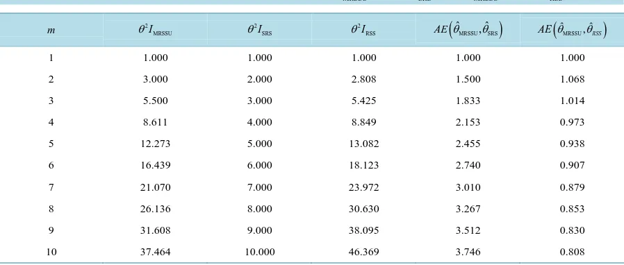
The numerical results are shown inTable 1. ARE of θˆMRSSU w.r.t. θˆSRS is greater than 1 and increases with

m. ARE of θˆMRSSU w.r.t. θˆRSS is greater than 1 for 1< ≤m 3 and decreases as m increases for m≥4. This is because RSS of the same size m uses more ranked units than MRSSU of the same size, for example RSS of size 5 uses 25 ranked units, whereas MRSSU of the same size uses only 15 ranked units.

5. Modified MLE (MMLE)

In order to obtain closed form approximate MLE of θ, the last term of LHS of likelihood Equation (2) is re-placed by its expectation. The idea of replacing the hazard rate in the maximum likelihood equation by its ex-pectation was proposed by Mehrotra and Nanda [10], who estimated parameters of normal and gamma distribu-tions based on Type II censored data. This technique used by Zheng and Al-Saleh [11] for obtaining MLE of location and scale parameters based on RSS.

Taking the expectation of third term of LHS of (2), we obtain

(

)

₂ 2

0 1

1 1

e 1 e d

i

x x

m

i

i i

x x

m

θ θ

θ

−

− −

∞

=

 

−

−

 

 

 

∑

∫

After simplification, we get likelihood Equation (2) as

(

)

( )

(

)

2

: 2

1 2 0

2 1 1

1 0

2

j

m m i

i i

i i j

i j

x i i

m m j

θ

θ −

= = =

−

 

−

 

 

− + − =

+

∑

∑

∑

Solving for θ, we have

: 1

ˆ m _,

i i i

d x m

θ =

=

∑

(11)

where

( )

(

)

( )

1 2

2 2 0

1 2

1

1 1 .

2

m i

j

i j

i i i

d

j

m j

− −

= =

 _{ −  − } _

 

= + _{  } − _  _ +   _



∑∑



ˆ

[image:5.595.89.538.526.717.2]

θ is called modified MLE of θ.

Table 1.The information numbers and asymptotic efficiencies of θˆMRSSU w.r.t. θˆSRS and θˆMRSSU w.r.t. θˆRSS.

m θ2IMRSSU

2 SRS I

θ 2

RSS I

θ AE

(

θˆMRSSU,θˆSRS

)

AE

(

θˆMRSSU,θˆRSS

)

1 1.000 1.000 1.000 1.000 1.000

2 3.000 2.000 2.808 1.500 1.068

3 5.500 3.000 5.425 1.833 1.014

4 8.611 4.000 8.849 2.153 0.973

5 12.273 5.000 13.082 2.455 0.938

6 16.439 6.000 18.123 2.740 0.907

7 21.070 7.000 23.972 3.010 0.879

8 26.136 8.000 30.630 3.267 0.853

9 31.608 9.000 38.095 3.512 0.830

Theorem 3.

a) ˆθ is unbiased estimator of θ.

b)

( )

(

)

( )

(

)

( )

2

2 2 1 1

2 3 2

1 0 1 0

1 1

ˆ

Var 2 1 1 ,

1 1

m i m i

j j

i j i j

i i

d i i

j j

m j j

θ

θ − −

= = = =  _{ −    −  }      = _{ } − − _{  } − _  _{+    +   }   

∑∑

∑ ∑

(12)

where d is defined as in Equation (11).

Proof a). From Equation (11), we have

( )

: 1 ˆ m i i i X E dE m θ =       =      

∑

i.e.,

( )

:

1 1 ˆ

m

i i i

X

E E

m d θ

=       =      

∑

(13)

It is well known that under some regularity conditions (see Lehmann [14] (pp. 440-441)), ∂L∗

( )

θ ∂ =θ 0. We can see that expectation of third term of Equation (2) simplifies to

( )

: : : 1 e 1 1

1 1 .

1 e i i i i X m i i X i X E i m d θ θ θ − − =      ₋ _{= −}     _{ }  −   

∑

(14)

Using Equation (13) and Equation (14), the expectation of Equation (2) reduces to

( )

1 _ˆ 1

1 0.

E

d d

θ− θ θ+ _ − =_

  (15)

Hence the proof of a).

Proof b). Since Xi i: is the i-th order statistics of a SRS of size i from the exponential distribution, with pa-rameter θ, the pdf of Xi i: is given by

( )

( )

₁

( )

1

( )

( )₁

: : :

0

1

, 1 e , 0, 0.

x

i _j

i j

i i i i i i

j

i i

g x i F x f x x

j θ θ θ θ − _{− +} − = −    

= _{ } = − _{ } > >  

∑

(16)

Now

( )

( )

( )

( )

( )

( )

(

)

(

)

( )

2

1 ₁ 1 ₁

2

: _{0 0}

0 0 2 1 1 2 3 2 0 0 1 1

Var 1 e d 1 e d

1 1

1

2 1 .

1 1

x x

i _j i _j

j j i i j j j i i j j j i i i i

X x x x x

j j

i i i

i j j j j θ θ θ θ θ − _{∞ − +} − _{∞ − +} = = − − = =   − −     = −   −   −         _{−  −    −  }   _{ }  = _{ }− _{ } −    _{+    +   }   

∑

∫

∑

∫

∑

∑

(17)

Thus using Equation (17), we obtain Equation (12).

We compare MMLE based on MRSSU relative to MLE using SRS and MMLE using RSS with the same size. From Equation (2.6) of Zheng and Al-Saleh [11] we can obtain MMLE of scale parameter of exponential distri-bution using RSS and is given by

(

)

( )

1 MMLE,RSS

1

ˆ m _{1 ,}

i i

d

m i x

m

θ

=

=

∑

− +

(

)

( )

(

)

1

2

1 2

2 0

2 1 1

1 1 .

2

j

m i

i j

i

m j

d i i

i

m m i j

−

−

= =

  −  ₋ 

 _{ }   

 

 

= +_{ −   }

− + +  

 

 

 

∑

∑

We can easily derive the variance of θˆMMLE,RSS and is given by

(

)

(

)

( )

(

)

( )

(

)

2

2 2 1 1

2 1

MMLE,RSS 2 3 2

1 0 0

1 1

1 1

ˆ

Var 1 2 .

1 1

j j

m i i

i j j

i i

m j m j

d

m i i i

i i

m m i j m i j

θ

θ − −

= = =

  _{ −    −  }    _{ }   −  _{ }   −            =  − +    −_   _ 

− + + − + +

   

 

 _{ } 

 

 

 _{   }

 

∑

∑

∑

Let e1 represents efficiency of MMLE ˆθ based on MRSSU w.r.t. θˆSRS based on SRS is given by

( )

( )

SRS 1

ˆ Var

. ˆ Var

e

θ θ

=

Similarly, efficiency of ˆθ relative to MMLE based on RSS is given by

(

)

( )

MMLE,RSS 2

ˆ Var

. ˆ Var

e θ

θ

=

The efficiencies were computed for m=1 1 10

( )

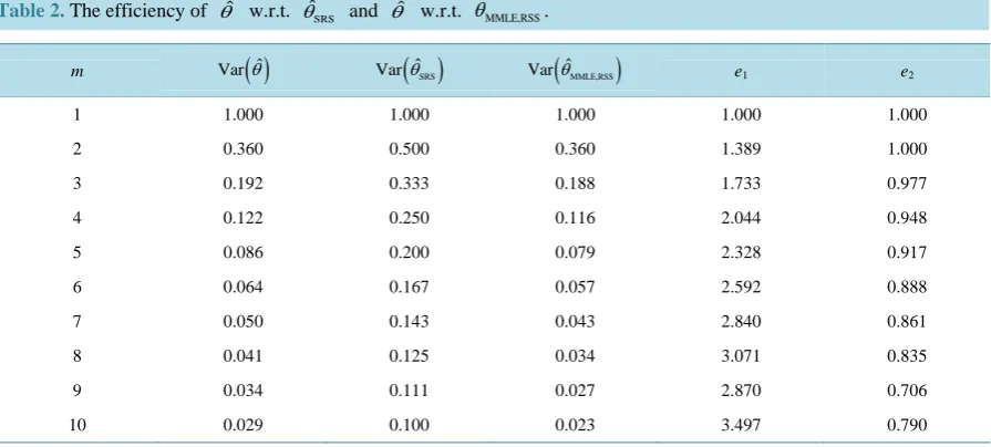
and are presented inTable 2. Note that the efficiency between any two of these estimators do not depend on θ and these values were computed only for θ=1. FromTable 2 it can be seen that computed efficiencies e1 increases as the sample size m increases. From e2 values we observed that estimator based on MRSSU are as efficient as estimator based on RSS for sample size m≤2, and then decreases for m≥3.

6. Errors in Ranking

In this section we study the situation where there are ranking errors. For MRSSU the ranking may not always be perfect, i.e., i-th largest observation in the i-th set measured by MRSSU method may not be the actual i-th larg-est order statistics in the set of size i. The errors in ranking may have an effect on the estimates.

[image:7.595.91.539.518.720.2]

To gain some insight of the effect of ranking errors on the efficiencies of the estimators, various simulation

Table 2.Theefficiency of _θˆ _w.r.t.

SRS ˆ

θ and _θˆ _w.r.t.

MMLE,RSS ˆ

θ .

m Var

( )

θˆ Var

( )

θˆSRS Var

(

θˆMMLE,RSS

)

e1 e2

1 1.000 1.000 1.000 1.000 1.000

2 0.360 0.500 0.360 1.389 1.000

3 0.192 0.333 0.188 1.733 0.977

4 0.122 0.250 0.116 2.044 0.948

5 0.086 0.200 0.079 2.328 0.917

6 0.064 0.167 0.057 2.592 0.888

7 0.050 0.143 0.043 2.840 0.861

8 0.041 0.125 0.034 3.071 0.835

9 0.034 0.111 0.027 2.870 0.706

trails were conducted. We use the simulation method considered by David and Lavine [15] and Dell and Clutter

[2]. In the first stage we generate m sets of simple random samples

{

Xi1,Xi2,,Xii

}

, i=1, 2,,m from the

exponential distribution with scale parameter θ=1. The corresponding m sets of random error variables

{

e ei1, i2,,eii

}

, i=1, 2,,m were generated from normal distribution with mean zero and variance

2

σ . De-fine

, 1, 2, , 1, 2, , ,

ij ij ij

Z =X +e i=  m j=  i

where Xij and eij are independent. Then we can obtain MRSSU’s of Xij’s and Zij’s (i=1, 2,,m, j=1, 2,,i).

The sets of

(

Z X_ij, _ij

)

i=1, 2,,m, j=1, 2,,i are ranked with respect to the first components of

(

Z_{( )i i:},X_{[ ]i i:}

)

. The second components are taken as judgment ranked order statistics and they constitute MRSSU’s with judg-ment error unless e_ij=0, i=1, 2,,m, j=1, 2,,i. We compute estimators ˆθ∗ based on judgment ranked MRSSU’s

{

X_{[ ]1 :1},X_{[ ]2 :2},,X_{[ ]m m:}

}

.

We repeat this procedure for 10,000 times. The estimate for θ is the average of the estimates from these replications, and variance of the estimate is the sample variance. Similarly using 10,000 simulated samples the RSS and SRS procedures were used to obtain the values of estimators of θ and their sampling variances. The simulated estimators based on RSS with imperfect ranking and SRS are denoted by θˆMMLE,RSS

∗

and θˆSRS

∗

. The efficiency and the expected value of the modified MLE ˆθ∗ have been computed by using R-software, version 3.0.2. The results are presented inTables 3-5.

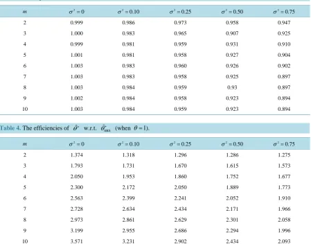
It is observed fromTable 3 that bias in the modified ML estimator ˆθ∗ ranges from 0.0002 to 0.1065, i.e., estimator based on ˆθ∗ is very close to true parameter. Based onTable 4 we can easily observe that the effi-ciency of the estimator based on ˆθ∗ w.r.t. estimator based on θˆSRS

∗

[image:8.595.90.540.358.710.2]

is larger than 1 and increases with m and

Table 3. The expectation values of _θˆ∗

(when θ=1).

m 2

0

σ = 2

0.10

σ = 2

0.25

σ = 2

0.50

σ = 2

0.75

σ =

2 0.999 0.986 0.973 0.958 0.947

3 1.000 0.983 0.965 0.907 0.925

4 0.999 0.981 0.959 0.931 0.910

5 1.001 0.981 0.958 0.927 0.904

6 1.003 0.983 0.960 0.926 0.902

7 1.003 0.983 0.958 0.925 0.897

8 1.003 0.984 0.959 0.93 0.897

9 1.002 0.984 0.958 0.923 0.894

10 1.003 0.984 0.959 0.923 0.894

Table 4. The efficiencies of _θˆ∗ _w.r.t.

SRS ˆ

θ∗ _{(when θ=1).}

m σ2=₀ σ =2 _0.10 σ =2 _0.25 σ =2 _0.50 σ =2 _0.75

2 1.374 1.318 1.296 1.286 1.275

3 1.793 1.731 1.670 1.615 1.573

4 2.050 1.953 1.860 1.752 1.677

5 2.300 2.172 2.050 1.889 1.773

6 2.563 2.399 2.241 2.052 1.910

7 2.728 2.634 2.434 2.171 1.966

8 2.973 2.861 2.629 2.301 2.058

9 3.199 2.955 2.686 2.294 1.996

[image:9.595.89.538.102.245.2]

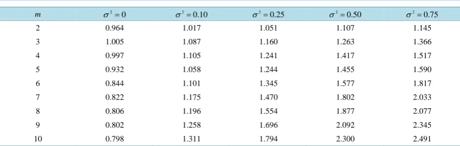
Table 5. The efficiencies of _θˆ∗ _w.r.t.

MMLE,RSS ˆ

θ∗

(when θ=1).

m 2

0

σ = 2

0.10

σ = 2

0.25

σ = 2

0.50

σ = 2

0.75

σ =

2 0.964 1.017 1.051 1.107 1.145

3 1.005 1.087 1.160 1.263 1.366

4 0.997 1.105 1.241 1.417 1.517

5 0.932 1.058 1.244 1.455 1.590

6 0.844 1.101 1.345 1.577 1.817

7 0.822 1.175 1.470 1.802 2.033

8 0.806 1.196 1.554 1.877 2.077

9 0.802 1.258 1.696 2.092 2.345

10 0.798 1.311 1.794 2.300 2.491

decreases with σ2 in the presence of ranking error. From Table 5 it can be seen that modified MLE based on ˆ

θ∗

w.r.t. θˆMMLE,RSS

∗

is larger than 1 and increases with m and σ2 in the presence of ranking error. This indi-cates that modified MLE ˆθ∗ based on MRSSU is better than modified MLE θˆMMLE,RSS

∗

in the presence of ranking error.

References

[1] McIntyre, G.A. (1952) A Method for Unbiased Selective Sampling Using Ranked Sets. Australian Journal of Agricul-tural Research, 3, 385-390. http://dx.doi.org/10.1071/AR9520385

[2] Dell, T.R. and Clutter, J.L. (1972) Ranked Set Sampling Theory with Order Statistics Background. Biometrics, 28, 545-555. http://dx.doi.org/10.2307/2556166

[3] Takahasi, K. and Wakimoto, K. (1968) On Unbiased Estimates of the Population Mean Based on the Sample Stratified by Means of Ordering. Annals of the Institute of Statistical Mathematics, 20, 1-31.

http://dx.doi.org/10.1007/BF02911622

[4] Lam, K., Sinha, B.K. and Wu, Z. (1994) Estimation of Parameters in Two-Parameter Exponential Distribution Using Ranked Set Sampling. Annals of the Institute of Statistical Mathematics, 46, 723-736.

http://dx.doi.org/10.1007/BF00773478

[5] Stokes, L. (1995) Parametric Ranked Set Sampling. Annals of the Institute of Statistical Mathematics, 47, 465-482. [6] Samwi, H., Ahmad, M. and Abu-Dayyeh, W. (1996) Estimating the Population Mean Using Extreme Ranked Set

Sam-pling. Biometrical Journal, 38, 577-586. http://dx.doi.org/10.1002/bimj.4710380506

[7] Al-Odat, M.T. and Al-Saleh, M.F. (2001) A Variation of Ranked Set Sampling. Journal of Applied Statistical Science, 10, 137-146.

[8] Al-Saleh, M.F. and Al-Hadrami, S. (2003a) Parametric Estimation for the Location Parameter for Symmetric Distribu-tions Using Moving Extremes Ranked Set Sampling with Application to Trees Data. Environmetrics, 14, 651-664.

http://dx.doi.org/10.1002/env.610

[9] Abu-Dayyeh, W. and Al Sawi, E. (2009) Modified Inference about the Mean of the Exponential Distribution Using Moving Extreme Ranked Set Sampling. Statistical Papers, 50, 249-259. http://dx.doi.org/10.1007/s00362-007-0072-5

[10] Mehrotra, K.G. and Nanda, P. (1974) Unbiased Estimator of Parameter by Order Statistics in the Case of Censored Samples. Biometrika, 61, 601-606. http://dx.doi.org/10.1093/biomet/61.3.601

[11] Zheng, G. and Al-Saleh, M.F. (2002) Modified Maximum Likelihood Estimators Based on RSS. Annals of the Institute of Statistical Mathematics, 54, 641-658. http://dx.doi.org/10.1023/A:1022475413950

[12] Al-Saleh, M.F. and Al-Hadrami, S. (2003b) Estimation of the Mean of the Exponential Distribution Using Moving Ex-tremes Ranked Set Sampling. Statistical Papers, 44, 367-382. http://dx.doi.org/10.1007/s00362-003-0161-z

[13] Chen, W.X., Xie, M.Y. and Wu, M. (2013) Parametric Estimation for the Scale Parameter for Scale Distributions Us-ing MovUs-ing Extremes Ranked Set SamplUs-ing. Statistics and Probability Letters, 83, 2060-2066.

http://dx.doi.org/10.1016/j.spl.2013.05.015

[14] Lehmann, E.L. (1983) Theory of Point Estimation. John Willey and Sons Inc., New York.

http://dx.doi.org/10.1007/978-1-4757-2769-2