2016 International Congress on Computation Algorithms in Engineering (ICCAE 2016) ISBN: 978-1-60595-386-1
1 INTRODUCTION
Hinterland was especially referred to the material distribution area around the harbor at first (Kong, 2007). Then, with the widely development the re-search content of economic geography, the concept of hinterland gradually was introduced into the layout research of the various economic center of the inland cities as well as the urban functional areas or facilities, so some scholars began to call it radiation scope, at-tracting scope or influencing scope. Due to the in-creasingly prominent role the logistics park played in regional economic development, the study of the defi-nition of its hinterland was also increased and, Zhang (2011) firstly defined the hinterland of the logistics park in his study. As the accurate definition the hin-terland of the logistics park provided the direct deci-sion making basis for the precise prediction of the logistics volume in the logistics park and the reasona-ble layout of function settings and scientific design for
the profit model, it was crucial for the rational, scien-tific and accurate planning of the entire logistics park project. With the advent of the information age, the technology that using GIS made spatial data analysis was developed and being applied, thus more and more scholars began using Voronoi diagram theory in computational geometry which had the advantage of the precise continuity in space-division to define hin-terland. Wang et al. (2002) firstly applied the Voronoi diagram theory to divide the urban influencing scope. Some subsequent scholars (Zhang et al., 2000, Wang, 2006 and Feng, 2010) extended its application to the influencing scope division of the urban public facili-ties and functional areas. Many scholars (Duan, 2010, and Huang et al., 1990) had combined the Voronoi diagram theory with the breaking-point model to cre-ate weighted Voronoi diagram theory which had more practical value and was tested well. However, the existing Voronoi diagram theory failed to fully reflect the impact of heterogeneity caused by the spatial me-dium on defining the hinterland. Therefore, based on the basic Voronoi diagram theory as well as fully
con-Definition of the Logistics Park Hinterland Based on the Analysis of
Spatial Medium Effect Applying to Weighted Voronoi Diagram
Haichao Nan*
Department of Railway Line & Station Design and Research, China Railway SIYUAN Design and Survey Group Co. LTD., Wuhan, Hubei, China
ABSTRACT: Accurately defining the logistics park hinterland is the basis of the rational planning of the logis-tics park as well as further improving the logislogis-tics efficiency. However, currently, the parameters of the methods and models for defining the logistics park hinterland are still not perfect, which lead those reasonableness and accuracy are also not ideal. Subsequently, based on the Voronoi diagram basic theory in computational geometry which reflects the advantage of the continuity of space division as well as by introducing both the ‘scale’ param-eter of the space object in the breaking-point model and the hparam-eterogeneity of the spatial medium caused by both the transportation network and the regional comprehensive strength factors into Voronoi diagram, the model based on the analysis of spatial medium effect applying to weighted Voronoi diagram to define the logistics park hinterland was built. Then the plug-in used in GIS software was programmed. Finally, this model and plug-in were practically applied to the planning example of Xinjin logistics park in Sichuan Province. Practice has proved that this model overcome the defects existing in the conventional space division theories and the ordinary Voronoi diagram theory, which makes the definition of the logistics park hinterland more reasonable and scien-tific.
Keywords: logistics park; Hinterland; Voronoi diagram; GIS
sidering the effect of the space object scale and the heterogeneity of the spatial medium caused by both the transportation network and the regional compre-hensive strength factors, the new method that weighted Voronoi diagram based on the analysis of spatial medium effect which was applied to defining the logistics park hinterland was proposed.
2 VORONOI DIAGRAM BASIC THEORY
In 1908, Voronoi diagram theory proposed by Russian mathematician M.G. Voronoi was used to divide spa-tial plane. In this theory, in any convex, Voronoi pol-ygon the distance that any point within some convex polygon from the space object within the convex pol-ygon is less than any point from any other space ob-jects in the spatial plane. Therefore, an important property of the Voronoi diagram is that the distance that each point within the Voronoi grid from the oc-currence point in the grid is less than that from any occurrence point in other Voronoi grids. Definition (1) represents the Voronoi diagram.
(1)
Where is the Voronoi diagram area of the space object pi; x is the set of space object stands for any point in the space; d is the Euclidean distance function.
Thereafter, since the Voronoi diagram had the ad-vantages of precise continuity in space division, many scholars gradually developed this theory. For example, both the variables such as the scale of the space object and traffic network that caused the heterogeneity of the spatial medium were respectively introduced into the Voronoi diagram theory to form weighted Voronoi diagram theory (Duan, 2010) and Voronoi diagram theory based on spatial network analysis(Lan, 2010); in addition, the two variables were simultaneously introduced into the Voronoi diagram theory to form the weighted Voronoi diagram theory based on spatial network analysis (Zhang, 2011). These theories had been applied to solving practical problems and achieved good results.
3 MODELING
3.1 Weighted Voronoi diagram based on the analysis of spatial medium effect
Although the weighted Voronoi diagram theory based on spatial network analysis improved the Voronoi diagram theory from the perspective of both the scale of the space object and traffic network that caused the heterogeneity of the spatial medium, it was still insuf-ficient in analyzing the factors caused the heterogene-ity of the spatial medium, namely, the differences
between existent different regions which caused the heterogeneity of the spatial medium were not taken into account. Therefore, the differences between ex-istent different regions were introduced into the fac-tors that caused the heterogeneity of the spatial me-dium, and then weighted Voronoi diagram based on the analysis of spatial medium effect was proposed in this study.
Suppose D = {P1 , P2 , P3 ,…, Pn} is the set of the
points on plane L. The network R = {l1, l2, l3,…, ln} is
composed of a variety of curve on plane L; R is an open network, namely, it can get free access to net-work R at any point; J = {G1, G2, G3,…, Gn} is a set of
the different regions on plane L, and Definition (2) is the weighted Voronoi diagram based on the analysis of spatial medium effect.
p
pd
xp
d
x p
i n
S j j tr i i tr i j i i n j
i
, 3 , 2 , 1 , , ,
(2)Where Sn (pi , λi) is the Voronoi diagram of space object pi ; P is the set of objectives; dtri is the dis-tance or time functions of objective pi based on the heterogeneity of the spatial medium caused by both the regional network and the regional comprehensive strength factors; t is the regional network factor; r is the existent regional differences factor; x is any point of space; λi is the weight of objective pi.
Definition (2) was introduced into the definition of logistics park hinterland to obtain Definition (3).
i nC p x d C p x d p C p S j j tr i i tr i j i i n j
i
, 3 , 2 , 1 , ,
,
(3)Where Sn (pi , Ci) is the Voronoi diagram of logistics park pi; P is the set of logistics parks;
i tr
d is the distance or time functions of logistics park pi based on the heterogeneity of the spatial medium caused by both the transport network and the regional compre-hensive strength factors; t is the transport network factor, which is determined by the relative speed of the different kinds or levels of roads compared with the non-transport network areas, as shown in Table 1; r is the existent regional differences factor, which is evaluated by index system established in Part 3.3; x is any point of space; Ci is the central strength of the logistics park pi , which is evaluated by index system established in Part 3.2.
3.2 Index system of evaluating the logistics park centrality
On the basis of the principles such as Macroscopic, comprehensiveness, operation and dynamic, the index system of evaluating the logistics park centrality was established in this study, as shown in Table 2.
xd x p dx p p p Pi j
pi i j i j
3.3 Index system of evaluating the regional compre-hensive strength
The regional comprehensive strength was also known as regional comprehensive competitiveness.
In this study, the comprehensive strength of the re-gion was illustrated by two aspects such as the scale of the economy and the quality of the economy, as shown in Table 3.
4 EXAMPLE
The method proposed in this study was used in this example to define the hinterland of Xinjin Logistics Park which was the key construction project of re-gional planning in Chengdu-Chongqing economic zone.
Based on the analysis of the existent logistics parks in Sichuan Province, the four logistics parks around
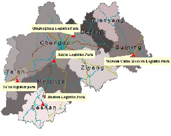
[image:3.516.55.459.69.102.2]and of the same level and type as Xinjin Logistics Park, namely, Jiazhou Logistics Park, Ya’an Logistics Park, Qingbaijiang Logistics Park and Western China Modern Logistics Park, as shown in Figure 1.
[image:3.516.55.469.127.280.2]Figure 1. Location of the logistics parks, transport network and regions. Table 1. Relative speed of the different kinds or levels of roads compared with the non-transport network areas. Roads level Railway Expressway National road Provincial road Non-transport network areas
Design real speed(km/h) 120 120 80 60 20
[image:3.516.59.461.305.451.2]Relative speed 6 6 4 3 1
Table 2. Index of evaluating the comprehensive strengths of the logistics parks.
Influencing factors Refinement index
Logistics park scale
Logistics gross product annually (X1) Investment intensity (X2)
Settled company qualification (X3) Whether it has bonded area (X4) Preferential policy (X5)
Equipment and facility of the logistics
Quality of equipment and facility (X6)
Information network level (X7) Multi-modal transport level (X8) Supporting services level (X9) Environmental level (X10) Service price level (X11)
Table 3. Index of evaluating the regional comprehensive strength.
Influencing factors Refinement index
Economy scale
Gross regional product (Y1)
Total retail sales of consumer goods (Y2)
Gross import and export (Y3)
Economy quality
Per capita GDP (Y4)
Average money wage of staff and workers (Y5) Per capita disposable income (Y6)
Per capita growth rate of social retailing consumer goods (Y7) Gross product in primary industry (Y8)
Gross product in secondary industry (Y9)
Gross product in tertiary industry (Y10)
[image:3.516.278.448.517.652.2]4.1 Evaluation of the logistics park centrality According to the index system of evaluating the logis-tics park centrality established in Table 1, the relevant original data was queried in statistics or obtained the experts grading, as shown in Table 4.
Table 4. Relevant original data of the index evaluating the regional comprehensive strength of the five logistics park.
(A)
Logistics parks
Index
X1 (10
2 million
Yuan)
X2 (10
2million
Yuan/mu) X3 X4 X5
A 200 0.005 4 2 4
B 60 0.004 3 1 3
C 233 0.005 4 1 4
D 25 0.01 3 2 4
E 500 0.01 4 1 4
(B)
Logistics parks Index
X6 X7 X8 X9 X10 X11
A 4 5 2 4 3 3
B 3 4 2 3 4 2
C 4 5 3 4 3 3
D 4 4 2 4 4 3
E 4 5 3 4 4 2
[image:4.516.53.254.153.318.2] [image:4.516.56.250.425.485.2]Then the principal component analysis was utilized to evaluate the original data by SPSS software. Ac-cording to the total variance explained table shown in Table 5 and based on the principle eigenvalues that are greater than 1 and the cumulative contribution rate which is more than 85%, the three main ingredients were determined.
Table 5. Total variance explained.
Component Initial Eigenvalues
Total % of Variance Cumulative %
1 5.515 50.140 50.140
2 2.967 26.971 77.111
3 2.028 18.433 95.544
4 .490 4.456 100.000
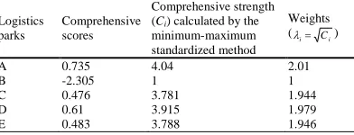
Then the scores of the principal components multi-plied the proportion that the corresponding eigenval-ues for each principal component accounted for the sum of all the principal components to get the com-prehensive evaluation scores. As the comcom-prehensive evaluation scores of some logistics parks calculated by SPSS were negative which could not be directly used in the model proposed in this study, Min-Max Nor-malization method as shown in Equation (4) was used to make the linear transformation of the original data which was mapped to the new data range〔1, 4.04〕to form the new data column, so the centrality of the logistics parks was obtained, as shown in Table 6.
A A
AA A
A
new new
new V
V _max _min _min
min max
min
'
(4)
Table 6. Comprehensive strengths of the five logistics parks.
Logistics parks
Comprehensive scores
Comprehensive strength (Ci) calculated by the
minimum-maximum standardized method
Weights (
i i C
)
A 0.735 4.04 2.01
B -2.305 1 1
C 0.476 3.781 1.944
D 0.61 3.915 1.979
E 0.483 3.788 1.946
Where V′is the data after normalization, V is the original data; max A and max B are respectively the maximum data and minimum data in original data column; new_ max A and new_ max B are respec-tively the maximum data and minimum data in new data column.
4.2 Evaluation of the comprehensive strength of the regions
According to the index system of evaluating the re-gional comprehensive strength established in Table 2, the relevant original data was queried in statistics, as shown in Table 7. Then the principal component analysis was utilized to evaluate the original data by SPSS software. According to the total variance ex-plained table shown in Table 8 and based on the prin-ciple eigenvalues that are greater than 1 and the cu-mulative contribution rate which is more than 85%, the main ingredients were determined. Then the scores of the principal components multiplied the proportion that the corresponding eigenvalues for each principal component accounted for the sum of all the principal components to get the comprehensive evaluation scores. As the comprehensive evaluation scores of some regions calculated by SPSS was negative which could not be directly used in the model proposed in this study, Min-Max Normalization method was used to make the linear transformation of the original data which was mapped to the new data range (1, 8.885) to form the new data column, so the centrality of the logistics parks was obtained, as shown in Table 9. Table 7. Relevant original data of the index evaluating the
regional comprehensive strength of the five logistics parks. (A)
Cities Index
Y1 (10
2
million Yuan)
Y2 (10
thou-sand Yuan)
Y3 (10
thou-sand dollars) Y4
(Yuan) Y5
(Yuan)
O 5551.33 24288296 2467759 41253 30515
P 921.27 3055028 223195 25335 28355
Q 960.22 4263018 159752 20053 26347
R 495.23 2084908 28150 14498 22621
S 657.90 2130041 15669 16644 24224
T 552.25 1885569 9985 18586 22897
U 286.54 1046540 1333 18881 23065
[image:4.516.263.465.532.672.2](B)
Cities Index
Y6 (Yuan) Y7 (%)
Y8 (10
2
million Yuan )
Y9 (10
2
million Yuan )
Y10 (10
2
million Yuan )
Y11
(%)
O 19920 18.6 285.09 2480.90 2785.34 65.51
P 16202 18.4 152.39 532.72 236.16 41.32
Q 15516 19.0 166.49 468.27 325.46 39.85
R 13778 17.4 109.39 254.69 131.15 38.38
S 15298 18.9 151.81 348.40 157.69 32.73
T 14644 17.8 103.80 303.31 145.14 34.11
U 14906 18.3 49.97 157.83 78.74 34.62
[image:5.516.265.463.123.275.2]V 15237 16.1 100.08 442.45 201.39 39.48
Table 8. Total variance explained.
Component Initial Eigenvalues
Total % of Variance Cumulative %
1 9.415 85.595 85.595
2 1.062 9.651 95.247
3 .308 2.802 98.048
4 .158 1.436 99.484
5 .051 .466 99.950
6 .004 .033 99.982
[image:5.516.54.254.216.305.2]7 .002 .018 100.000
Table 9. Regional comprehensive strength of the cities.
Cities Comprehensive scores
Comprehensive strength (ri) calculated by the
minimum-maximum standardized method
Weights (
i r )
Chengdu(O) 6.289 8.885 2.981
Deyang(P) 0.237 2.833 1.683
Mianyang(Q) -0.103 1.651 1.285
Suining(R) -1.576 1.225 1.107
Ziyang(S) -0.935 2.493 1.579
Meishan(T) -1.371 1.02 1.01
Ya’an(U) -1.596 1 1
Leshan(V) -0.945 1.661 1.289
4.3 Definition of the hinterland of Xinjin Logistics Park
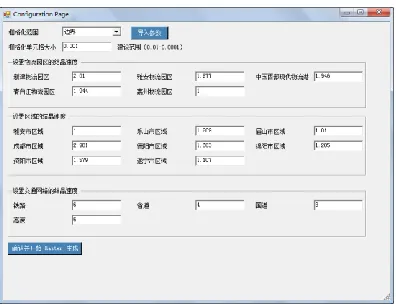
On the basis of the crystal growth algorithm, by using ArcObjects development tools and C# programming software to implement the secondary development, the plug-in of weighted Voronoi diagram based on the analysis of spatial medium effect that could be directly installed into ArcMap for operation was generated, as shown in Figure 2. In addition, this plug-in had the characteristics of simple operation and universality, because it can load the file with precise location in-formation including Shape and Dwg format as well as directly import the relevant parameters from Excel.
With this plug-in, the related layers were loaded in-to Arcmap. Meanwhile, the parameters calculated in Parts 4.1 and 4.2 were also imported to obtain the definition result, which showed the hinterland of Xin-jin Logistics Park covered the western and southern region of Chengdu City, the southwestern and central
region of Meishan City, the northern region of Ya’an City and the northeastern region of Leshan, as shown in Figure 3. Finally, “Calculate Geometry” tool in Arcmap was used to calculate the area of the hinter-land of Xinjin Logistics Park which was 10,885.46 square kilometers.
[image:5.516.279.443.316.456.2]Figure 2. The plug-in of weighted Voronoi diagram based on the analysis of spatial medium effect in ArcMap.
Figure 3. Diagram of the hinterlands of Xinjin Logistics Parks.
5 CONCLUSION
[image:5.516.51.254.335.441.2]method to define the logistics park hinterland, the dividing line was put in the first place, so when the Voronoi diagram formed was not a completely closed space, this method was also subject to certain limita-tions. In a word, these deficiencies need to be further studied in the future.
REFERENCES
[1] Kong, X. B. 2007. Study on city’s economic hinterland and it’s spatial definition-take Chengdu and Mianyang as examples. Chengdu: Southwest Jiaotong University. [2] Zhang, Y. B. 2011. Research on the method of defining
logistics park hinterland-weighted Voronoi diagram based on transportation network. Chengdu: Southwest Jiaotong University.
[3] Wang, X. S., Li, Q. & Guo, Q. S. 2002. The generaliza-tion and construcgeneraliza-tion of Voronoi diagram and its appli-cation on delimitating city’s affected coverage. Journal of Central China Normal University (Natural Sciences)
36(1): 107-110.
[4] Zhang, L., & Zhou, H. Y. 2004. Research on public es-tablishment location selection based on the Voronoi dia-gram in GIS. Computer Engineering and Applications,
(9): 223-227.
[5] Wang, Y. F. 2006. GIS and Voronoi Polygon based pub-lic health care accessibility analysis. Geomatics &
Spa-tial Information, 29(3): 77-80.
[6] Feng, S. M. 2010. Study on service coverage of distribu-tion center based on Voronoi diagram. Areal Research
and Development, 29(3): 142-144.
[7] Duan, Q. L. 2010. Spatial scope and the layer of nan-jing’s economic hinterland based on breaking point the-ory. Resources and Environment in the Yangtze Basin,
19(8): 853-858.
[8] Huang, J. Y., Zhang, P. Y. & Liu, Y. 1990. The change of urban economic influence regions in Heilongjiang province since 1990. Economic Geography, 30(7): 1118-1123.