Improved tests for spatial autoregressions

(1)

Autoregressions

Francesca Rossi

Dissertation submitted for the degree of

Doctor of Philosophy in Economics at

The London School of Economics and Political Science

(2)

Declaration

I certify that the thesis I have presented for examination for the PhD degree of the London School of Economics and Political Science is solely my own work other than

where I have clearly indicated that it is the work of others.

The copyright of this thesis rests with the author. Quotation from it is permitted, pro-vided that full acknowledgment is made. This thesis may not be reproduced without

the prior written consent of the author.

I warrant that this authorization does not, to the best of my belief, infringe the rights

of any third party.

(3)

Abstract

Econometric modelling and statistical inference are considerably complicated by the possibility of correlation across data data recorded at different locations in space. A

major branch of the spatial econometrics literature has focused on testing the null

hypothesis of spatial independence in Spatial Autoregressions (SAR) and the asymp-totic properties of standard test statistics have been widely considered. However, finite

sample properties of such tests have received relatively little consideration. Indeed,

spatial datasets are likely to be small or moderately-sized and thus the derivation of finite sample corrections appears to be a crucially important task in order to obtain

reliable tests. In this project we consider finite sample corrections based on formal

Edgeworth expansions for the cumulative distribution function of some relevant test statistics.

In Chapter 1 we provide the background for the results derived in this thesis. Specifically, we describe SAR models together with some established results in first

order asymptotic theory for tests for independence in such models and give a brief

account on Edgeworth expansions. In Chapters 2 and 3 we present refined proce-dures for testing nullity of the spatial parameter in pure SAR based on ordinary

least squares and Gaussian maximum likelihood, respectively. In both cases, the

Edgeworth-corrected tests are compared with those obtained by a bootstrap proce-dure, which is supposed to have similar properties. The practical performance of new

tests is assessed with Monte Carlo simulations and two empirical examples. In

Chap-ter 4 we propose finite sample corrections for Lagrange Multiplier statistics, which are computationally particularly convenient as the estimation of the spatial parameter is

not required. Monte Carlo simulations and the numerical implementation of Imhof’s

procedure confirm that the corrected tests outperform standard ones. In Chapter 5 the slightly more general model known as “mixed” SAR is considered. We derive suitable

finite sample corrections for standard tests when the parameters are estimated by

or-dinary least squares and instrumental variables. A Monte Carlo study again confirms that the new tests outperform ones based on the central limit theorem approximation

(4)

(5)

Acknowledgments

First of all, I am greatly indebted to my advisor, Professor Peter Robinson, for his invaluable support and guidance.

Many thanks are due to Abhisek Banerjee, Zsofia Barany, Ziad Daoud, Abhimanyu

Gupta, Javier Hidalgo, Tatiana Komarova, Jungyoon Lee, Oliver Linton, Elena Man-zoni, Myung Hwan Seo, Marcia Schafgans and Sorawoot Tang Srisuma for plenty of

helpful comments and discussions.

I also thank all my friends and fellow researchers at the LSE, in particular the participants at the work in progress seminars, for discussions and comments on my

work.

Financial support from the Bank of Italy, Fondazione Luigi Einaudi and ESRC Grant RES-062-23-0036 is gratefully acknowledged.

I owe a lot to my family, and in particular to my parents, for their support over the past few years, and to Antonio, for being so patient and supportive. All this would

not have been possible without them.

(6)

List of Figures

2.1 Simulated pdf ofaˆλunderH0 in (1.2.1) . . . 43

2.2 Simulated pdf ofg(aλˆ) underH0 in (1.2.1) . . . 43

3.1 Simulated pdf of ˜a˜λunderH0 in (1.2.1) . . . 68

(9)

List of Tables

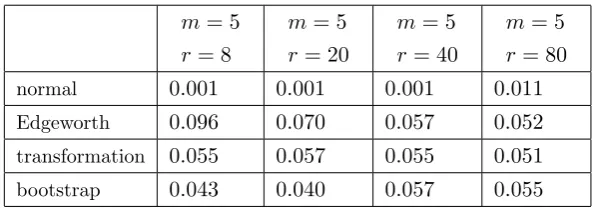
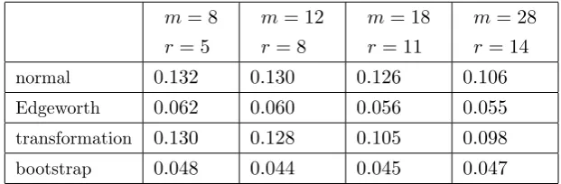
2.1 Empirical sizes of the tests of H0 in (1.2.1) againstH1 in (2.1.1) whenλin model

(1.2.5) is estimated by OLS and the sequencehis “divergent”. The reported values have to be compared with the nominal 0.05.. . . 42 2.2 Empirical sizes of the tests ofH0 in (1.2.1) againstH1 in (2.1.1) whenλin model

(1.2.5)is estimated by OLS and the sequencehis “bounded”. The reported values have to be compared with the nominal 0.05.. . . 42 2.3 Empirical sizes of the tests of H0 in (1.2.1) againstH1 in (2.2.1) whenλin model

(1.2.5) is estimated by OLS and the sequencehis “divergent”. The reported values have to be compared with the nominal 0.05.. . . 44 2.4 Empirical sizes of the tests of H0 in (1.2.1) againstH1 in (2.2.1) whenλin model

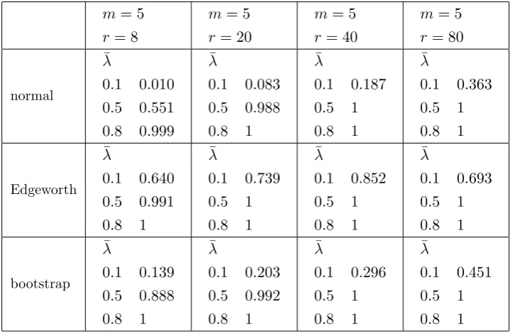
(1.2.5)is estimated by OLS and the sequencehis “bounded”. The reported values have to be compared with the nominal 0.05.. . . 44 2.5 Empirical powers of the tests of H0 in (1.2.1) against H1 in (2.5.3), with ¯λ =

0.1,0.5,0.8, when λ in model (1.2.5) is estimated by OLS and the sequence h is “divergent”. αis set to 0.95. . . 45 2.6 Empirical powers of the tests of H0 in (1.2.1) against H1 in (2.5.3), with ¯λ =

0.1,0.5,0.8, when λ in model (1.2.5) is estimated by OLS and the sequence h is “bounded”. αis set to 0.95. . . 45 2.7 Numerical values corresponding to (2.5.5) (second row) and (2.5.6) (third row),

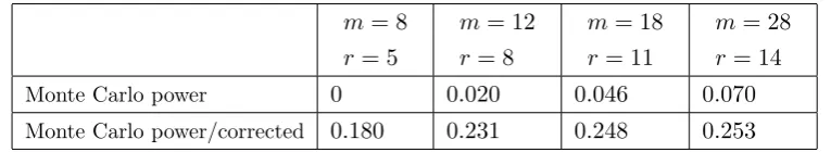
com-pared with the simulated values for the power of a test of (1.2.1) against (2.4.1) when λn in model (1.2.5) is estimated by OLS and the sequencehis “divergent”. . . 46 2.8 Numerical values corresponding to (2.5.5) (second row) and (2.5.6) (third row),

com-pared with the simulated values for the power of a test of (1.2.1) against (2.4.1) when λn in model (1.2.5) is estimated by OLS and the sequencehis “bounded”. . . 47 2.9 Simulated values of the power of a test of (1.2.1) against (2.4.1) based on the standard

and corrected statistics when λn in model (1.2.5) is estimated by OLS and the sequencehis “divergent”. The values should be compared with the target 0.304. . 47 2.10 Simulated values of the power of a test of (1.2.1) against (2.4.1) based on the standard

and corrected statistics when λn in model (1.2.5) is estimated by OLS and the sequencehis bounded. The values should be compared with the target 0.304.. . . 48 3.1 Empirical sizes of the tests ofH0 in (1.2.1) whenλin (1.2.5) is estimated by MLE

and the sequence his “divergent”. The reported values have to be compared with the nominal 0.05. . . 67 3.2 Empirical sizes of the tests ofH0 in (1.2.1) whenλin (1.2.5) is estimated by MLE

and the sequenceh is “bounded”. The reported values have to be compared with the nominal 0.05. . . 67 3.3 Empirical powers of the tests of H0 in (1.2.1) against H1 in (2.5.3) with ¯λ =

(10)

3.4 Empirical powers of the tests ofH0 in (1.2.1) against (2.5.3) with ¯λ= 0.1,0.5,0.8

when λin (1.2.5) is estimated by MLE and the sequencehis “bounded”. αis set to 0.95. . . 70 3.5 Outcomes of the tests ofH0 in (1.2.1) whenλin model (3.3.2) is estimated by OLS 72 3.6 Outcomes of the tests ofH0 in (1.2.1) whenλin model (3.3.2) is estimated by MLE 72 3.7 Outcomes of the tests ofH0 in (1.2.1) whenλin model (3.4.1) is estimated by OLS 74 3.8 Outcomes of the tests ofH0 in (1.2.1) whenλin model (3.4.1) is estimated by MLE 74 4.1 Empirical sizes of the tests of (1.2.1) against (2.2.1) for model (1.2.5) when the

sequencehis “divergent”. The reported values have to be compared with the nominal 0.05. . . 103 4.2 Empirical sizes of the tests of (1.2.1) against (2.2.1) for model (1.2.5) when the

sequencehis “bounded”. The reported values have to be compared with the nominal 0.05. . . 103 4.3 Empirical sizes of the tests of (1.2.1) against (2.2.1) for model (1.2.15) when the

sequencehis “divergent”. The reported values have to be compared with the nominal 0.05. . . 104 4.4 Empirical sizes of the tests of (1.2.1) against (2.2.1) for model (1.2.15) when the

sequencehis “bounded”. The reported values have to be compared with the nominal 0.05. . . 104 4.5 Edgeworth-corrected and Imhof’sα-quantiles of the cdf ofT in whenhis “divergent”.108 4.6 Edgeworth-corrected and Imhof’sα-quantiles of the cdf ofT whenhis “bounded”. 108 5.1 Empirical sizes of the tests of (1.2.1) against a one-sided alternative when λandβ

in (1.1.3) are estimated by OLS. The reported values have to be compared with the nominal 0.05. . . 133 5.2 Empirical sizes of the tests of (1.2.1) against a one-sided alternative when λandβ

in (1.1.3) are estimated by IV. The reported values have to be compared with the nominal 0.05. . . 133 5.3 Empirical sizes of the tests of (5.3.1) withR= (0,1)0against a one-sided alternative.

λand βin (1.1.3) are estimated by IV and λ= 0.1,0.7. The reported values have to be compared with the nominal 0.05. . . 134 5.4 Empirical sizes of the tests of (5.3.1) withR= (−1,1)0against a one-sided

(11)

1 Introduction

This chapter provides the background to appreciate the specific contribution of

this thesis to the existing spatial econometric literature and the main theoretical techniques we will employ. Specifically, in Section 1.1 we discuss some issues that

arise with spatial data, together with a description of spatial autoregressions. In

Section 1.2 we give an account of established first order asymptotic theory for testing for lack of correlation in spatial autoregressions. In Section 1.3 we report an overview

on Edgeworth expansions and their application to derive improved tests, while in

Section 1.4 we describe the motivation of this thesis, in view of some of the existing results discussed in Sections 1.2 and 1.3. Finally, in Section 1.5 we introduce some

definitions and assumptions that will be used in Chapters 2-5.

1.1 Spatial Autoregressions

Econometricians face considerable challenges posed by the possibility of

cross-sectional correlation, with respect to both modelling and statistical inference. Indeed,

starting from the early work by Moran (1950), Cliff and Ord (1968, 1972) and, more recently, Cressie (1993), just to name a few, a large body of literature known as

Spatial Econometrics has addressed issues entailed by potential correlation across

data recorded at different locations in space. For recent reviews and discussions of the challenges and progresses in the spatial econometric literature, refer to Robinson

(2008a) and Anselin (2010).

Much of the spatial statistical literature has focused on data recorded on a lattice, i.e. regularly-spaced observations on ad−dimensional space, where d >1. In general, intervals between observations are constant within dimensions, but are allowed to vary

across different dimensions. Some extensions of standard asymptotic theory for the time series setting (d = 1) to the case d > 1 are possible, as first noted by Whittle (1954). Indeed, Whittle (1954) demonstrates that, in general, multilateral models have

a “half-plane” type of unilateral moving average representation which extends the well known Wold representation for time series data, and hence suggests estimates of the

underlying unknown parameters based on an approximation for the Gaussian

log-likelihood function. However, such half-plane representations might contain functions of the coefficients of the multilateral model that cannot be expressed in closed form.

Furthermore, a serious source of complication arising with lattice data ford >1 is the bias of the estimates entailed by the “edge effect”. Techniques to overcome such bias

are developed in Guyon (1982), Dahlhaus and K¨unsh (1987) and Robinson and Vidal

Sanz (2006).

However, observations recorded on a lattice are very uncommon in economics.

For example, in geographical settings there is irregular spacing when observations are

(12)

spaced geographical locations, a generalisation of the established theory for irregularly-spaced time series is still possible. Specifically, some cases of irregularly-irregularly-spaced time

series can be described by an underlying continuous time process where spacing is

generated by a point process. When the continuous time process is a first order stochastic differential equation with constant coefficients and driven by white noise,

consistent and asymptotically normal estimates of the unknown parameters can be

obtained from an approximated Gaussian log-likelihood (see Robinson (1977)). This framework can in principle be extended to more general models, but estimation and

asymptotic theory become complicated.

In any case, “space” should be more generally intended as a network, which in-cludes physical/geographical space as a very special case, and in turn correlation

across observations may depend on some very general notion of economic distance

(e.g. differences in household income) that does not necessarily have a geographical interpretation (see e.g. Conley and Ligon (2002) or Conley and Dupor (2003)). The

economic distance between units (or economic agents) i and j is defined as the dis-tance between ui and uj, whereui and uj are vectors of characteristics pertaining to

agents i and j, respectively. The distance between ui and uj might be defined in an

Euclidean sense. The aforementioned extensions of the theory for irregularly-spaced

time series to spatial data are unsuitable in case there is no geographical aspect. Spatial autoregressions (SAR) offer a useful, applicable framework for describing

such data. In SAR models the notion of possible irregular spacing, applied to general

economic distances, is embodied in an n×n weight matrix (n being sample size), denoted Wn, which needs to be chosen by the practitioner. Let wij be the (i, j)−th

element of Wn. Conventionally, wii = 0 fori= 1, ....n, i.e. the spatial interaction of

each unit (or economic agent) with itself is set to zero. Although in principle wij can

be negative, in most practical applications Wn has non negative entries and is row

normalized, so that elements of each row sum to 1. In view of such normalization,wij

can be defined in terms of the inverse of an economic distancedij between unitsiand

j, i.e.

wij =

dij n

P

s=1

dis

, (1.1.1)

wheredij ≥0 and possiblydij 6=dji, i.e. symmetry of the spatial interaction between

unitsiand j (or economic agents iand j) is not imposed.

For instance, when the data are recorded across different regions or countries Wn

can be chosen according to a contiguity criterion, i.e. wij = 1 if regions or countries

share a border and wij = 0 otherwise. Eventually, the resulting matrix can then be

the row normalized so that

n

P

j=1

wij = 1 for all i. Alternatively, wij can be defined as

inverse of the geographical distance (e.g. measured in miles of kilometers) between

locations i and j. In such case, the resulting Wn is not row normalized. In the

(13)

former specification, i.e. based on a contiguity criterion and then row normalized. An example of Wn, introduced by Case (1991), that has been extensively used to

illustrate theoretical results is

Wn=Ir⊗Bm, Bm=

1 m−1(lml

0

m−Im), (1.1.2)

where n = rm, r being the number of districts and m the number of households in each district. In (1.1.2), ⊗ indicates the Kronecker product, lm an m−dimensional

column of ones andIr ther×ridentity matrix. Henceforth, we retain the subscript to

eitherl orI only when the dimension is other thann, i.e. throughout land I denote an n−dimensional column of ones and then×nidentity matrix. Under (1.1.2), two households are neighbours if they belong to the same district, and each neighbour is given the same weight. Since Wn in (1.1.2) is symmetric and block diagonal, (1.1.2)

is a convenient choice computationally and hence it has often been adopted in Monte

Carlo simulations to illustrate theoretical results. Indeed, throughout this thesis we will employ (1.1.2) for our simulation studies. It should be stressed that although

(1.1.2) has been introduced by Case (1991) in a geographical setting, the block diagonal structure of (1.1.2) can be used to describe more general situations where each unit

(agent) is equally influenced by units (agents) with similar characteristics and is not

affected by other units (agents) in the economy.

Although the choice of Wn plays a central role in deriving asymptotic theory for

spatial data and is a crucial empirical issue, we should outline that in this thesis we

will deal with tests for spatial independence and most of our results are derived under the null hypothesis of no spatial correlation. For this reason, our results would be

valid even in case Wn is not correctly chosen. However, efficiency of tests is affected

by the choice ofWn.

Let Yn be an n×1 vector of observations, Xn an n×k matrix of exogenous

regressors of full column rank which might include a column of ones, and n an n×1

vector of independent and identically distributed (iid) random variables, with mean zero and unknown varianceσ2. We assume that, for some unknown scalarλand some unknownk×1 vector β, the data follow a general SAR model, i.e.

Yn=λWnYn+Xnβ+n. (1.1.3)

For notational simplicity, in the sequel we drop thensubscript, writing=n, Y =Yn,

X=Xn,W =Wn,with the same convention for othern−dependent quantities.

Model (1.1.3) is a very parsimonious method of describing spatial dependence,

con-veniently depending only on economic distances rather than actual locations, which

may be unknown or not relevant. For sake of clarity, it should be stressed that often in the spatial econometric literature “spatial independence” is used as a synonym for

(14)

Gaussianity. Although a major drawback of SAR models is the ex ante specification of W, to which parameter estimates are sensitive, (1.1.3) has been widely used in practi-cal applications. Relevant book-length descriptions of SAR model and its applications

include Anselin (1988) and Arbia (2006). Even more importantly, (1.1.3) represents a convenient, widely-usable class of alternatives in testing the null hypothesis of lack

of spatial correlation which, if true, considerably simplifies statistical inference. Much

of the results in this thesis (Chapters 2, 3 and 4) are derived under the assumption that β= 0 a priori in (1.1.3), or thatX =l, i.e. (1.1.3) only contains an intercept.

Although in this thesis we will only deal with SAR models, we acknowledge that

an interesting alternative approach to describe spatial interactions based on economic distances has been formulated by Conley (1999). In Conley (1999), economic agents’

observations are modelled as realizations of a random process at points of a Euclidean

space and the distance between two agents in such Euclidean space reflects their proximity (economic distance). Under mixing conditions and in a random field setting,

Conley (1999) derives asymptotic theory for various estimates. Conley (1999) and

Conley and Molinari (2007) also extend such a framework in case of measurement error in the economic distance.

1.2 First order statistics

The problem of testing the null hypothesis

H0:λ= 0 (1.2.1)

in (1.1.3), or in a related model where the spatial correlation potentially also affects

the unobservable disturbances, i.e.

Yn=λWn,1Yn+Xnβ+un un=ρWn,2un+n, (1.2.2)

Wn,1 and Wn,2 being suitable weight matrices and ρ a scalar parameter, is a long

lasting issue in the spatial econometric literature.

When the focus of the investigation is both on estimation and testing ofλin models (1.1.3) or (1.2.2) various tests of (1.2.1) based on different estimates of λhave been proposed and widely used by practitioners. Ordinary Least Squares (OLS) estimation

ofλandβ in (1.1.3) was dismissed without thorough investigation in early work since W Y in (1.1.3) is correlated withand hence OLS estimates are generally inconsistent. However, Lee (2002) shows that OLS estimates ofλandβ in (1.1.3) can be consistent and asymptotically normal for some choices of W. Throughout, the OLS estimates of λand β are denoted by ˆλand ˆβ, respectively. Let h=hn be a sequence bounded

away from zero for all n. For wij given in (1.1.1) and such that n

P

s=1

(15)

bounded away from zero at rate h, i.e. for alln

0< c1 < n

P

s=1

dis

h ,

where√n/h=o(1) andc1 being a generic arbitrarily small constant, Lee (2002) shows

that as n→ ∞,

√

n(ˆλ−λ,( ˆβ−β)0)0→d N(0, VOLS), (1.2.3) d

→ and prime indicating convergence in distribution and transposition, respectively, and

VOLS =σ2 lim

n→∞

1 n

E(Y0)W0 X0

!

(W E(Y), X) !−1

.

In caseh diverges at rate √n, Lee (2002) shows

√

n(ˆλ−λ,( ˆβ−β)0)0 →d N(b, VOLS), (1.2.4)

where b is an asymptotic bias that vanishes only when λ = 0. Such results do not hold in case h/√n =o(1). Although t-type of tests of (1.2.1) based on ˆλ and ˆβ are computationally very simple, the aforementioned strong condition onW restricts their applicability.

Lee (2002) also shows that in case β in (1.1.3) is zero a priori, i.e. when the data follows a “pure” SAR

Y =λW Y +, (1.2.5)

ˆ λ= Y

0_W0_Y

Y0W0W Y (1.2.6)

is inconsistent and more generally, the estimate of λis inconsistent when (1.1.3) only includes an intercept. However, in each of these cases, under H0 in (1.2.1), the OLS

estimate ofλactually does converge to zero in probability. Although the caseλ= 0 is very limited when the interest is estimation, it is a leading one in testing and we will

consider it in detail in Chapter 2. We will also show that when the data are driven by (1.2.5), underH0 in (1.2.1), the rate of convergence of ˆλmight be slower than the

parametric √n, depending on assumptions onW.

Procedures based on Gaussian maximum likelihood estimates (MLE) for λ and β in (1.1.3) and (1.2.2) have been developed by Cliff and Ord (1975) and broadly considered. For an exhaustive survey about specification and implementation of tests of (1.2.1) based on the Gaussian MLE of parameters in (1.1.3) and (1.2.2), refer

to Anselin (1988). Asymptotic properties of MLE and Pseudo-MLE (i.e. estimates

obtained by maximization of a Gaussian log-likelihood function when normality of the error terms is not assumed) of λ,β and σ in (1.1.3), denoted ˜λ, ˜β, ˜σ henceforth, and relevant test statistics have been derived in Lee (2004). Henceforth PMLE indicates

(16)

The pseudo log-likehood function of (1.1.3) is defined as

l(λ, β, σ2) =−n

2ln(2π)− n 2lnσ

2₊_{ln(det(S(λ)))}₋ 1

2σ2(S(λ)Y −Xβ)

0_(S(λ)Y ₋_Xβ),

(1.2.7) where, for every value ofλ,

S(λ) =I−λW (1.2.8)

anddet(A) denotes the determinant of a generic square matrixA. It should be stressed that in (1.2.7), λ, β and σ denote any admissible value of the parameters in (1.1.3). Givenλ, the PMLE of β and σ2 are

˜

β(λ) = (X0X)−1X0S(λ)Y (1.2.9)

and

˜

σ2(λ) = 1 n(Y

0_S(λ)0₋_β_˜_(λ)0_X0_)(S(λ)Y ₋_X_β(λ)),_˜ _(1.2.10)

respectively. Hence

˜

λ= arg max

λ∈Λ l(λ,

˜

β(λ),σ˜2(λ)), (1.2.11) where Λ is a compact set included in (−1,1). The PMLE ofβ andσ2 are then defined as ˜β = ˜β(˜λ) and ˜σ2= ˜σ2(˜λ).

In particular, assuming wij = O(1/h), h being either divergent or bounded and

such thath/n→0 as n→ ∞, Lee (2004) proves that under standard conditions,

√

n(˜λ−λ,( ˜β−β)0)0 →d N(0, VP M LE), (1.2.12)

where the explicit form of VP M LE is given in Lee (2004) and is not reported here in

order to avoid introducing further unnecessary notation. It should be stressed that whenβ6= 0 and the elements ofare normally distributed,VP M LE =VOLS. Although

estimation of λ in (1.2.5) can be regarded as a constraint maximization of (1.2.11) when β= 0, Lee (2004) shows that in this case

r n h ˜

λ→d N(0, V_{P M LE}pure ), (1.2.13) where V_{P M LE}pure denotes the asymptotic variance of pn/hλ˜ in case the data follow (1.2.5). From (1.2.13) it is clear that the rate of convergence of ˜λtoλ can be slower than√nwhen his divergent. Test statistics based on ˜λwhen the data are driven by (1.2.5) will be the focus of Chapter 3.

Although the MLE (or PMLE, more generally) has been extensively used for both

(17)

(1998) and subsequently improved by Lee (2003).

In particular, Kelejian and Prucha (1998) derive asymptotic properties of IV

esti-mates of parameters in (1.2.2). Although Kelejian and Prucha (1998) show consistency

and asymptotic normality of IV estimates of λ and β, denoted ˆλIV and ˆβIV

hence-forth, in the more general model (1.2.2), we report here only their results pertaining

to (1.1.3). LetZbe an×(k+ 1) matrix of instruments. Under standard assumptions, Kelejian and Prucha (1998) prove

√

n(ˆλIV −λ,( ˆβIV −β)0)0 d

→N(0, VIV), (1.2.14)

where

VIV =σ2

lim

n→∞

1 nZ

0_{(W E(Y}_{), X)}

−1 lim

n→∞

1 nZ

0_Z

lim

n→∞

1 n

E(Y0)W0 X0

! Z

!−1

The latter result holds under very weak conditions onW, and more details about those will be provided in Chapter 5. The “ideal” choice of instruments isZ = (W E(Y), X) and with such choiceVIV =VOLS. Also, with such choice forZand under normality of

the error terms,VIV =VM LE. Kelejian and Prucha (1998) propose to approximate the

“ideal” instrument, which is clearly infeasible, with a subset of the linearly independent

columns of (X, W X, W2X, ...). However, Kelejian and Prucha (1998) do not consider relative efficiency issues and, in general, their choice ofZ is suboptimal.

In turn, Lee (2003), improves the asymptotic efficiency of the Kelejian and Prucha

IV estimator. In a more recent paper, Kelejian et al. (2004) introduce a series-type IV estimator for model (1.2.2), which is proved to be asymptotically normal, efficient

within the class of IV estimators and computationally simpler than one proposed in

Lee (2003).

We should mention that, although the test of (1.2.1) is generally the main focus,

we might be interested in testing restrictions onβ in (1.1.3) and (1.2.2). However, IV estimates cannot be obtained in caseβ = 0 in (1.1.3) and (1.2.2) and hence tests for the joint significance of β1, ....βk (βi being thei−th element ofβ) are not possible in

this setting.

In Chapter 5 we will focus on tests for λand β in (1.1.3) based on ˆλIV and ˆβIV,

starting from Kelejian and Prucha (1998) main framework.

On the other hand, when the interest of the practitioner is testing rather than estimation, a class of tests based on Langrange Multiplier (LM) statistics has received

considerable attention starting from the early contribution by Moran (1950). Such

tests are computationally very convenient as the estimation ofλin either model (1.1.3) or (1.2.2) is not required.

Moran (1950) presents a simple correlation test between neighbours in space based

(18)

(1972, 1981) to test H0 in (1.2.1) in regression models with SAR disturbances, i.e.

Y =Xβ+u, u=λW u+. (1.2.15)

(1.2.15) is equivalent to (1.2.2) whenλin (1.2.2) is zero a priori, but we separate the two models to outline clearly whether the parameter that we wish to test is the SAR coefficient when the disturbances are also potentially correlated (i.e. λin (1.2.2)) or that of the disturbance term of a linear regression (i.e. λ in (1.2.15)). In particular, assuming normality of the components of in (1.2.15), Cliff and Ord (1972) show that Moran’s statistic under H0 in (1.2.1) has a χ21 asymptotic distribution . Cliff

and Ord’s (1972) normality assumption has been relaxed by Sen (1976), who derives

theχ2₁ asymptotic distribution of Moran’s test forH0 in (1.2.1) when the data follow

(1.2.15) assuming that the components of are iid and under some specific moment conditions. Though Moran test statistic (and its aforementioned extensions) was not

originally derived in a ML framework, Burridge (1980) shows it is indeed equivalent to a LM statistic for spatially uncorrelated disturbances. Details of LM statistics to

test H0 in (1.2.1) will be given below.

Although this is not explicitly considered in this thesis, Kelejian and Robinson

(1992) derive an alternative test for spatial independence against correlation of

un-specified form in the disturbance term of regression models (possibly nonlinear) based on regression residuals. Kelejian and Robinson (1992) do not refer explicitly to a

weight matrix and the ordering of observations is based on first order contiguity.

Sim-ilarly to Moran’s, Kelejian and Robinson test has a χ2 limiting distribution under (1.2.1) and its asymptotic properties have been derived without assuming normality

of the error terms. However, the small sample performance of Kelejian and Robinson

test is quite poor, as shown in a number of Monte Carlo studies (e.g. Anselin and Florax (1995) and Kelejian and Robinson (1998)).

Anselin (2001) provides an exhaustive survey of derivation and implementation

issues of Moran/LM tests of (1.2.1) when the data follow either (1.1.3) or (1.2.2). As regarding asymptotic theory of Moran/LM test statistics, Kelejian and Prucha

(2001) derive a central limit theorem for quadratic forms in random variables which

allows to establish the asymptotic distribution of LM statistics for SAR models under H0 in (1.2.1). This result is general enough to accommodate non linearity and the

possibility of heteroskedastic error terms. Also, Pinske (1999, 2004) outlines a set of

conditions for asymptotic normality (or asymptotic χ2) of several Moran/LM-type of test statistics, which include LM statistics for testing (1.2.1) in (1.1.3), (1.2.2) and

(1.2.15).

We briefly outline here some details on the construction of a version of the LM statistic to test H0 in (1.1.3), its modification to either (1.2.2) or (1.2.15) is

(19)

defined as

LM =

∂l(λ, β, σ2) ∂λ |H0

2

−E

∂2l(λ, β, σ2) ∂λ2

|_H₀

−1

. (1.2.16)

From (1.2.7), by standard partial differentiation,

∂l(λ, β, σ2)

∂λ |H0 =n ˆ 0W Y

ˆ 0ˆ ,

where ˆ=Y −Xβˆr and ˆβr is the OLS estimate ofβ in (1.1.3) underH0 (“restricted”

model, hence the superscript “r”) in (1.2.1) . Similarly,

−E

∂2l(λ, β, σ2) ∂λ2 |H0

=tr(W2) +tr(W0W) +n(W X ˆ

βr)0P W Xβˆr) ˆ

0_ˆ ,

where

P =I−X(X0X)−1X (1.2.17)

and trindicates the trace operator. The derivation of (1.2.16) is based on a Gaussian likelihood but the same first order limit distribution obtains more generally. Indeed, as anticipated, under suitable conditions we have

LM →d χ2₁. (1.2.18)

Tests of (1.2.1) based on (1.2.16) (or its appropriate modification) for either (1.2.5) or (1.2.15) will be considered in detail in Chapter 4.

More generally, Robinson (2008b) derives the asymptotic distribution under the

null hypothesis of lack of correlation of a class of residual-based test statistics, which include LM for either (1.1.3) or (1.2.2) as special cases. As expected, by considering

the asymptotic distribution of such residubased class of statistics under a local

al-ternative, LM tests are motivated because they are locally optimal within this class. Finite sample improvements of test statistics under the null hypothesis of lack of

cor-relation are also suggested. Robinson (2008b) results will be presented and discussed in detail in Chapter 4.

1.3 Edgeworth expansions

In Section 1.2 we mentioned which test statistics will be considered in Chapters

2-5. However, before illustrating more precisely the contribution of this thesis, in this section we give a brief account of existing literature on Edgeworth expansions, which

are indeed the main methodological instruments for the derivation of our results.

The literature on Edgeworth expansions and their applications in econometric and statistical theory is very broad and here we only aim to provide some of the main

(20)

develop this project, although we acknowledge that this is not a complete survey. The idea of (formally) expanding distribution functions was introduced by

Edge-worth (1896, 1905) for sums of iid random variables. For useful and relatively simple

surveys which deal with the derivation of Edgeworth expansions, refer to Rothenberg (1984) and Barndorff-Nielsen and Cox (1989, Chapter 4). Here, we illustrate briefly

the derivation of the Edgeworth expansion for the cumulative distribution function

(cdf) of the standardized sample mean of iid random variables and how such deriva-tion can be extended to the case of quadratic statistics in normal random variables,

which are the main focus of this thesis.

Specifically, letU1, U2, ...Unbe a sample of iid random variables with meanm= 0

and varianceV ar(Ui) = 1. It is well known that the sample mean

¯

Un= ¯U =

1 n

n

X

i=1

Ui

is a √n−consistent estimate of m. For notational simplicity, letSn =S =

√

nU¯. By the central limit theorem,

S→d N(0,1).

Equivalently, the latter result can be expressed in terms of the characteristic function

of S, i.e.

E eitS

→e−t2/2

asn→ ∞, wheree−t2/2 is the characteristic function ofN(0,1) and i=√−1. However, we might be interested in improving upon the approximation offered by

the central limit theorem. Letκp be thep−th cumulant ofUi (throughout this thesis,

κpwill denote thep−th cumulant of various quantities and the reader will be reminded

of this in each specific case in order to avoid notational confusion). It is known that

the cumulant generating function of Ui,ψUi(t), can be written as an infinite series in κp, i.e.

ψUi(t) =

∞

X

p=1

(it)p p! κp.

Since κ1 =m= 0 and κ2 =V ar(Ui) = 1, the latter expression becomes

ψUi(t) =− 1 2t

2₊ ∞

X

p=3

(it)p

p! κp. (1.3.1)

From (1.3.1), the cumulant generating function ofS,ψS(t), can be derived as

ψS(t) =nψUi(t/

√

n) =−1

2t

2₊ ∞

X

p=3

(it)p

np2−1p!

(21)

From (1.3.2), it is clear that the normalized cumulants of S,

n−p2+1κ_p forp≥3, are decreasing in p. Hence, from (1.3.2),

E eitS=eψS(t) ₌_e

−1₂t2₊P∞

p=3 (it)p n

p 2−1p!

κp

=e−12t 2

 1 +

∞

X

p=3

(it)p

np2−1p! κp+

1 2   ∞ X p=3 (it)p

np2−1p! κp   2 +...  

=e−12t 2

1 +√1

n (it)3

6 κ3+ 1 n

(it)4

24 κ4+ (it)6 72 κ 2 3 +...

=e−12t 2

1 +√1

nR1(it) + 1

nR2(it) +...

, (1.3.3)

where

R1(it) =

(it)3 6 κ3, R2(it) =

(it)4 24 κ4+

(it)6 72 κ

2 3

and so on.

Since

e−12t 2

= Z

<

eitxdΦ(x), (1.3.4)

Φ(x) being the standard normal cdf, (1.3.3) suggests the “inverse” expansion

P r(S ≤x) = Φ(x) +√1

nP1(x) + 1

nP2(x) +.... (1.3.5) wherePj(x) denotes a function whose Fourier-Stieltjes transform is Rj(it)e−t

2_/₂ , i.e.

Z

<

eitxdPj(x) =Rj(it)e−t

2_/₂ .

By repeated integration by parts of (1.3.4),

Pj(x) =Rj(−d/dx)Φ(x), (1.3.6)

where d/dx denotes the differential operator and Rj(d/dx) should be interpreted as

a polynomial in d/dx. For notational compactness, throughout we denoteg(i)(x) the i−th derivative of a function g. From (1.3.6), (1.3.5) becomes

P r(S ≤x) = Φ(x)−√1

n 1 6κ3Φ

(3)_{(x) +}1

n

1 24κ4Φ

(4)_{(x) +} 1

72κ

2

3Φ(6)(x)

(22)

The latter is called Edgeworth expansion of the cdf of S.

Generally, (1.3.7) is truncated after a certain number of terms, e.g.

P r(S ≤x) = Φ(x)−√1

n 1 6κ3Φ

(3)_{(x) +}1

n

1 24κ4Φ

(4)_{(x) +} 1

72κ

2

3Φ(6)(x)

+O

1 n3/2

, (1.3.8)

where the order of the remainder is conjectured from the rate and the parity of the coefficients. Such argument is purely formal. It is possible to prove validity of (1.3.8)

by deriving the order of the remainder uniformly for all x. Starting from the work developed by Cram´er (1946), Sargan (1976) and Bhattacharya and Ghosh (1978), among others, provided rigorous theory for validity of formal Edgeworth expansions. A

seminal book-length account of Edgeworth expansions and rigorous results for validity

issues is Bhattacharya and Rao (1976). In this thesis, we rely on formal Edgeworth expansions and validity proofs are left for future work.

As anticipated at the beginning of this section, this thesis will mainly deal with

quadratic statistics in normal random variables and hence a short digression on how to extend the derivation of the Edgeworth expansion described above for the cdf ofS to quadratic forms in normal random variables is worthwhile here. The characteristic function of a quadratic form0C, where the elements ofare iid, normally distributed with mean zero and varianceσ2andCis an×nsymmetric matrix, can be analytically evaluated by Gaussian integration as

E(eit0C) = 1 (2πσ2₎n/2

Z

<

e− ξ0ξ 2σ2eitξ

0_Cξ

dξ

= 1

(2πσ2₎n/2

Z

<

e−

ξ0(I−2itC)ξ

2σ2 dξ=det(I−2itC)−1/2. (1.3.9)

From (1.3.9), the cumulant generating function and hence the cumulants of 0C can be derived. Once such cumulants are known, after suitable algebraical manipulation, we can write an expansion for the characteristic function of a standardized version

of 0C, similar to one given in (1.3.3), and hence derive the corresponding Edge-worth expansion for the cdf. The derivation of EdgeEdge-worth expansions for the cdf of quadratic forms in normal random variables will be discussed thoroughly in the proofs

of Theorems of Chapters 2-5.

It is clear that (1.3.8) (or a similar expansion for the statistic of interest) provides

a more accurate approximation of the cdf ofS(or of the cdf of the statistic of interest) than one offered by the central limit theorem. Also, (1.3.8) can be used to derive a better approximation for the quantiles of the cdf ofS than one based on the quantiles of the standard normal. Alternatively, starting from (1.3.8), it is possible to derive a

transformed statisticg(S) so that its cdf is closer to the normal than that ofS. Such results are very useful to derive improved testing procedures, since the former gives

(23)

the latter provides improved test statistics under the null hypothesis. Obviously, these results extend to the case of statistics other than S and the derivation of such Edgeworth-corrected critical values and Edgeworth-corrected test statistics will be

shown and discussed in detail in this thesis in case of quadratic test statistics in normal random variables.

Several authors have applied Edgeworth expansions to derive refined test statistics

in several context, starting from the work on the inverse of Edgeworth expansions by Cornish and Fisher (1937, 1960). Among these, Konishi et al (1988) derive the

Edgeworth expansion and Edgeworth-corrected quantiles for the cdf of quadratic forms

in normal random variables. Taniguchi (1986, 1988, 1991a, 1991b), derives higher order asymptotic properties of test statistics for time series data. Other relevant

examples of derivation of refined test statistics in time series contexts include Magee

(1989) and Kakizawa (1999). More specifically, Magee (1989) develops Edgeworth-corrected tests for linear restrictions when the data follow a linear regression with

serially correlated disturbances. Also, Kakizawa (1999), starting from the earlier

work by Ochi (1983), derives a valid Edgeworth expansion for the cdf of two different estimates of the correlation parameter in first order autoregressions and hence provides

Edgeworth-corrected confidence intervals. In a different context, Phillips and Park

(1988) derive Edgeworth-corrected Wald tests of nonlinar restrictions.

Before concluding this account on Edgeworth expansions, we should mention that

Hall (1992) offers a very useful monograph which gives a view of the theory on

Edge-worth expansions and EdgeEdge-worth-corrected tests in order to explain the performance of bootstrap methods. Indeed, it is well established, starting from the work by Singh

(1981), that the bootstrap is a technique that can be used instead of the analytical derivation of Edgeworth expansions to improve upon the approximation offered by the

central limit theorem. Indeed, Singh (1981) shows that the bootstrap automatically

corrects for the first term after the normal cdf in an Edgeworth expansion (e.g. the second term at the RHS of (1.3.8)).

Although we do not aim to show theoretically the equivalence between the first

Edgeworth correction and the bootstrap, in this thesis we compare by Monte Carlo the practical performance of Edgeworth corrections with bootstrap-based procedures

and more specific references to relevant bootstrap literature will be given in Chapters

2-5.

1.4 Finite sample issues and contribution of this thesis

In Section 1.2 we provided an account of existing tests for (1.2.1) in SAR models,

while in Section 1.3 we introduced the Edgeworth expansions and briefly discussed how they can be used to derive improved tests. Indeed, the main scope of this thesis is to

derive refined tests for (1.2.1) in SAR models based on formal Edgeworth expansions.

(24)

in (1.2.5) based on ˆλand ˜λ, respectively. The refined tests derived in Chapters 2 and 3 will also be applied in two small empirical examples. In Chapter 4 we will derive

improved LM tests of (1.2.1) in (1.2.5) and (1.2.15). In Chapter 5 we will derive

Edgeworth-corrected tests for (1.2.1) in (1.1.3) based on ˆλand ˆλIV. Although testing

for spatial independence is the main focus of this work, in Chapter 5 improved tests

for linear restrictions on β in (1.1.3) based on ˆβIV are also derived. Small sample

performance of Edgeworth-corrected tests are assessed by Monte Carlo and compared with bootstrap-based procedures.

This thesis is motivated by the fact that although the literature on testing for

spatial independence is very broad, analytical derivation of finite sample corrections for such tests has received little attention, other than the aforementioned

contribu-tion by Robinson (2008b). This issue is of particular concern in spatial econometrics

since datasets are usually small/moderately-sized, as very often the practitioner is interested in estimating and testing spatial coefficients of SAR models when data are

recorded across cities, regions of countries. For instance, the two empirical examples

considered in this thesis deal with spatial correlation of variables recorded across 43 European countries and 103 Italian regions, respectively (hence n= 43 and n= 103, respectively). When n is small/moderately-sized, testing procedures based on the normal (orχ2) approximation for the distribution of test statistics might be seriously unreliable.

Together with the likely limited sample size, another source of concern for the

reliability of standard testing procedures in SAR models is given by the possibly slow rate of convergence of ˆλ and ˜λ when the data follow (1.2.5), as outlined in Section 1.2. When this is the case, the cdf of statistics based on such estimates is poorly approximated by a normal and finite sample corrections are indeed crucial in order

to obtain reliable tests. This issue provide even stronger motivation for the new tests

presented in Chapters 2 and 3.

Although the spatial econometrics literature on analytical finite sample corrections

is very limited, small sample performance of estimates of the parameters in (1.1.3),

(1.2.2) and (1.2.15) and corresponding tests have been assessed quite extensively by Monte Carlo studies, see e.g. Anselin and Rey (1991), Anselin and Florax (1995),

Das et al. (2003) and, more recently, Egger et al. (2009). More specifically, Anselin

and Rey (1991) and Anselin and Florax (1995) report and discuss broad sets of Monte Carlo results to evaluate the practical performances of various existing tests for spatial

independence. Das et al. (2003) perform a Monte Carlo study to assess the finite

sample behaviour of IV-type of estimates of parameters in (1.2.2), while Egger et al. (2009) propose a similar analysis for Wald-type of tests of (1.2.1) in SAR models based

on MLE and Generalized Method of Moments estimates.

(25)

function, they derive the second order bias and mean squared error of ˜λ in (1.2.5). However, Bao and Ullah (2007) do not outline the possibly slow rate of convergence

of ˜λin (1.2.5) and do not consider improved tests.

1.5 Some definitions and Assumptions

We first define some notation that will be used throughout and has not been introduced previously.

i) φ(z) denotes the the probability density function (pdf) of a standard normal random variable.

ii) 1(.) indicates the indicator function, i.e. 1(A ⊂ B) = 1 if A ⊂ B and 1(A ⊂

B) = 0 otherwise.

iii) Hj(x) denotes thej−th Hermite polynomial, i.e.

Hj(x) = (−1)jex

2_/₂ dj dxje

−x2_/₂

, (1.5.1)

e.g.

H1(x) =x, H2(x) =x2−1 and H3(x) =x3−3x.

iv) ∼ denotes an exact rate, i.e. a ∼ b means that |a/b| converges to a positive, finite limit.

v) ηi(A),i= 1, ....q denotes the eigenvalues of a genericq×q matrixA.

vi)

¯

η(A) = max

i=1,....q{|ηi(A)|}. (1.5.2)

vii)

η

−

(A) = min

i=1,....q{|ηi(A)|}.

viii) ||.||indicates the spectral norm, i.e. for any p×q matrixB

||B||2 _{= ¯}_η(B0_B).

ix) ||A||r denotes the maximum row sum matrix norm, i.e.

||A||_r= max

i q

X

j=1

|aij|,

(26)

x) ||A||c indicates the maximum column sum matrix norm, i.e.

||A||c= max j

q

X

i=1

|aij|.

We introduce some assumptions, which are common to Chapters 2-5, while other relevant model-specific conditions are left to each chapter.

Assumption 1 The elements of are independent and identically distributed normal random variables with mean zero and unknown variance σ2.

Assumption 2

(i) For all n, wii= 0, Σnj=1wij = 1,i= 1, ..., n, and ||W||= 1.

(ii) For all n, W is uniformly bounded in row and column sums in absolute value, i.e.

||W||r+||W||c≤K,

where K is a finite generic constant.

(iii) Uniformly in i, j = 1, ..., n,wij =O(1/h), where h=hn is bounded away from

zero for all nand h/n→0 as n→ ∞.

As is common in much higher order literature, Gaussianity is assumed in this

derivation. Assumption 1 can be relaxed at expense of considerable extra

complica-tions in the derivation of Edgeworth expansions. We should stress that Assumption 1 is not necessary for (1.2.3), (1.2.4), (1.2.12), (1.2.13), (1.2.14) and (1.2.18) which

indeed hold more generally. However, in this thesis we are interested in deriving

statistics with better finite-sample properties and we can only justify these under the precise distributional assumption.

The normalizations in Assumption 2(i) are not strictly necessary for the proofs

of the results presented in Chapters 1-4, but they play a role in constructing the likelihood. Furthermore, Assumption 2(i) or some other normalization is required for

identification whenλ6= 0. Assumption 2(i) requires thatW is row normalized so that the elements in each row sum to one. It also imposes that the maximum eigenvalue of W0W equals one. It should be stressed that actually ||W||= 1 would be sufficient for identification purposes and hence row normalization seems somehow redundant. However, the latter entails significant algebraical simplifications in the derivation of

some of the results presented in this thesis (see e.g. Section 2.3) and is therefore

(27)

Assumption 2(ii) is standard. It has been introduced by Kelejian and Prucha (1998) to keep the spatial correlation to a manageable degree. Assumption 2(ii) plays

an important role both in the proofs of the first order theory results, i.e. (1.2.3),

(1.2.4), (1.2.12), (1.2.13), (1.2.14) and (1.2.18) and in the proofs of the results of this thesis. It is also worth mentioning that row normalization and non negative wij, for

all i, j= 1, ...., n, implies||W||_r = 1.

Assumption 2(iii) formalises the definition and some general conditions on the se-quence h already introduced in Section (1.2). Indeed, Assumption 2(iii) is the same as one in Lee (2004). As already outlined in Section 1.2, h can be bounded or di-vergent. A condition onwij is commonly required in asymptotic theory for statistics

based on SAR models. Assumption 2(iii) will be suitably strengthened in Chapter 5,

consistently with one in Lee (2002), as discussed in Section 1.2.

(28)

2 Improved OLS Test Statistics

for Pure SAR

Throughout most of this chapter we assume that for some scalar λ∈(−1,1) the data follow (1.2.5), which is model (1.1.3) when β = 0 a priori, i.e. none of the exogenous regressors is relevant, and we are interested in testing (1.2.1) when λ is estimated by OLS. An extension of the proposed procedures to the pure SAR with

intercept term is also considered.

As discussed in Chapter 1, it is known (Lee (2002)) that ˆλ in model (1.2.5) is inconsistent when λ 6= 0. However, it converges to zero in probability under (1.2.1) and although this case is limited when the interest is estimation, it is relevant in testing

and should be investigated further. As anticipated in Chapter 1, in this chapter we show that, underH0 in (1.2.1), the rate of convergence of ˆλmight be slower than the

parametric √n, depending on assumptions onW.

When the rate of convergence of ˆλ is slower than √n, the cdf of the t-statistic based on ˆλunder (1.2.1) is not accurately approximated by a normal. Our new tests are based on refined t-statistics, whose cdf are closer to the normal than those of

the standard statistics and therefore entail better approximations. Alternatively, we show that inference based on standard statistics can be improved by considering more

accurate approximations for critical values than ones of the normal cdf.

This chapter is organised as follows. In Sections 2.1 and 2.2 we present refined tests for (1.2.1) against one-sided and two-sided alternatives, respectively. In Section 2.3,

we show that the results of Sections 2.1 and 2.2 can be easily extended when model (1.2.5) contains a location parameter. In Section 2.4 we present some results for the

power of the test of (1.2.1) against a local alternative. In Section 2.5 we report and

discuss the results of some Monte Carlo simulations of the tests presented in Sections 2.1-2.4. Relevant proofs are left to appendices.

2.1 Test against a one-sided alternative: Edgeworth-corrected criti-cal values and corrected statistic

We suppose that model (1.2.5) holds and we are interested in testing (1.2.1) against

a one-sided alternative

H1 :λ >0 (<0). (2.1.1)

As previously mentioned, ˆλ in (1.2.6) converges in probability to zero under H0, as

(29)

Assumption 3The limits lim n→∞ h ntr(W 0

W), lim

n→∞

h

ntr(W W

0

W), lim

n→∞

h ntr((W

0

W)2), lim

n→∞

h ntr(W

2_), _lim

n→∞

h ntr(W

3₎ _(2.1.2)

are non-zero.

Under Assumption 2 the limits displayed in (2.1.2) exist and are finite by Lemma 2.1. Thus, the content of Assumption 3 is that such limits are also non-zero. Letζ be any finite real number.

Theorem 2.1 Let model (1.2.5) and Assumptions 1-3 hold. The cdf of λˆ under H0 in (1.2.1) admits the third order formal Edgeworth expansion

Pr(aˆλ≤ζ|H0) = Φ(ζ) + 2bζ2φ(ζ)−

κc₃ 3!Φ

(3)_(ζ₎₋

tr((W0W)2) (tr(W0_W₎₎2 −6b

2

ζ3φ(ζ)

+ 2b2ζ4Φ(2)(ζ)−κ

c 3

3 bζ

2_Φ(4)_{(ζ) +} κc4

4!Φ

(4)_{(ζ) +}_O

h n

3/2! , (2.1.3)

where

a= tr(W

0_W₎

(tr(W0_W ₊_W2₎₎1/2, b=

tr(W W0W)

(tr(W0_W ₊_W2₎₎1/2_tr(W0_W₎, (2.1.4)

κc₃ ∼ 2tr(W

3_{) + 6tr(W}0_W2₎

(tr(W0_W ₊_W2₎₎3/2 (2.1.5) and

κc₄ ∼ 6tr(W

4_{) + 24tr(W}0_W3_{) + 12tr((W W}0₎2_{) + 6tr(W}2_W02₎

(tr(W0W +W2₎₎2 . (2.1.6)

The proof of Theorem 2.1 is in the Appendix.

Under Assumption 3, as n→ ∞

b∼

h n

1/2

, tr((W

0_W₎2₎

(tr(W0_W₎₎2 ∼

h n, κ

c 3 ∼

h n

1/2

, κc₄ ∼ h

n and therefore

2bζ2φ(ζ)−κ

c 3

3!Φ

(3)_(ζ)_∼

h n

1/2 ,

−

tr((W0W)2) (tr(W0W))2 −6b

2

ζ3φ(ζ) + 2b2ζ4Φ(2)(ζ)−κ

c 3

3 bζ

2_Φ(4)_{(ζ) +}κc4

4!Φ

(4)_(ζ)_∼ h

(30)

Since a∼(n/h)1/2 from Assumption 3, when the sequence h is divergent the rate of convergence of P r(aλˆ ≤ ζ|H0) to the standard normal cdf is obviously slower than

the usual √n. It must be stressed that the expansion in (2.1.3) is formal and hence the order of the remainder can only be conjectured by the rate of the coefficients.

As anticipated in Chapter 1, from the expansion (2.1.3) Edgeworth-corrected

crit-ical values can be obtained. We denotewα andzα theα−quantiles of the null statistic

aˆλand the standard normal cdf, respectively. By inversion of (2.1.3) we can obtain an infinite series forwα, i.e.

wα =zα+p1(zα) +p2(zα) +..., (2.1.7)

where p1(zα) and p2(zα) are polynomials of orders (h/n)1/2 and h/n, respectively.

Both p1(zα) and p2(zα) can be determined using the identity α = P r(aˆλ≤ wα|H0)

and the asymptotic expansion given in Theorem 2.1. Even though the procedure can

be extended to higher orders, for algebraic simplicity we focus on the second order Edgeworth correction and therefore only p1(zα) has to be determined.

For convenience, we report the second order Edgeworth expansion

Pr(aλˆ≤ζ|H0) = Φ(ζ) + 2bζ2φ(ζ)−

κc₃ 3!Φ

(3)_(ζ_{) +}_O

h n

. (2.1.8)

From (2.1.8) and the property (derived from (1.5.1))

(−d/dx)jΦ(x) =−Hj−1(x)φ(x), (2.1.9)

we have

α= Pr(aλˆ≤wα|H0) = Φ(wα)−(

κc₃

3!H2(wα)−2bw

2

α)φ(wα) +O

h n

.

Moreover, expandingwα according to (2.1.7) and dropping negligible terms,

α = Pr(aλˆ≤wα|H0)

= Φ(zα) +p1(zα)φ(zα)−(

κc₃

3!H2(zα)−2bz

2

α)φ(zα) +O

h n

= α+p1(zα)φ(zα)−(

κc₃

3!H2(zα)−2bz

2

α)φ(zα) +O

h n

, (2.1.10)

where the second equality follows by Taylor expansion of Φ(wα) aroundzα. The last

displayed identity holds up to orderO(h/n) when

p1(zα) =

κc₃

3!H2(zα)−2bz

(31)

Hence (2.1.7) becomes

wα =zα+

κc₃

3!H2(zα)−2bz

2

α+O

h n

. (2.1.11)

The size of the test of (1.2.1) obtained with the usual approximation of wα byzα,

that is

P r(aλ > zˆ α|H0), (2.1.12)

can be compared with the one obtained using the Edgeworth-corrected quantile as

given in (2.1.11), i.e.

P r(aλ > zˆ α+

κc₃

3!H2(zα)−2bz

2

α|H0). (2.1.13)

When zα is used to approximatewα, the error has order (h/n)1/2,while it is reduced

to (h/n) when the Edgeworth-corrected critical value is used.

Rather than corrected critical values, an Edgeworth-corrected test statistic can be

derived. By (2.1.9) and sinceH2(ζ) =ζ2−1, (2.1.8) can be written as

Pr(aˆλ≤ζ|H0) = Φ(ζ+ 2bζ2−

κc₃ 3!(ζ

2₋_{1)) +}_O

h n

.

When the transformation

v(ζ) =ζ+ 2bζ2−κ

c 3

3!(ζ

2₋_{1) =}_ζ_{+ (2b}₋κc3

3!)ζ

2₊κc3

3!

is monotonic, we can write

Pr(aλˆ+ (2b−κ

c 3

3!)(aλ)ˆ

2₊κc3

3! ≤ζ) = Φ(ζ) +O

h n

and make inference on λbased on the corrected statisticv(aˆλ). The function v(ζ) is strictly increasing whenζ > −1/(2(2b−κc₃/3!)), however the latter does not hold in general and therefore a cubic transformation that does not affect the remainder but

such that the resulting function is strictly increasing over the whole domain should be considered. A suitable transformation is in Hall (1992) or, in a more general case,

Yanagihara et al (2005):

g(ζ) =v(ζ) +Q(ζ), with Q(ζ) = 1 3

2b−κ

c 3

3! 2

ζ3.

Indeed, it can be shown (Yanagihara et al (2005)) that for a statisticT that admits the general expansion

P r(T ≤x) = Φ(x) +p1(x)φ(x) +O

h n

(32)

wherep1(x)∼

p

h/n, the transformation

g(x) =x+p1(x) +

1

4Q(x) with Q(x) = Z

d dxp1(x)

2

dx (2.1.14)

is strictly increasing and does not affect higher order terms, i.e.

P r(g(T)≤x) = Φ(x) +O

h n

.

It is straightforward to verify that in the present case the function g(ζ) is strictly increasing for every ζ,its first derivative being (1 + (2b−(κc₃/3!)ζ))2.

The size of the test of (1.2.1) based on such corrected statistic,

P r(g(aλ)ˆ > zα|H0), (2.1.15)

can be compared with the standard (2.1.12). As previously mentioned, the error

when the standard statistic is used has orderph/n, while it is reduced to h/n when considering the corrected variant.

2.2 Test against a two-sided alternative: Edgeworth-corrected criti-cal values and corrected statistic

In Section 2.1 we focused on testing (1.2.1) against (2.1.1). However, in some circumstances the practitioner might not have a prior conjecture about the sign of λ in (1.2.5) and a test of (1.2.1) against a two-sided alternative may be more suitable. In this section we propose refined tests for (1.2.1) against a two-sided alternative

H1 :λ6= 0. (2.2.1)

From Theorem 2.1, (2.1.9) and

φ(−ζ) =φ(ζ), Φ(2)(−ζ) =−Φ(2)(ζ), Φ(3)(−ζ) = Φ(3)(ζ), Φ(4)(−ζ) =−Φ(4)(ζ), we obtain

P r(|aλˆ| ≤ζ|H0) = P r(aλˆ≤ζ)−P r(aˆλ≤ −ζ)

= Φ(ζ)−Φ(−ζ)−2

tr((W0W)2) (tr(W0_W₎₎2 −6b

2

ζ3φ(ζ) + 4b2ζ4Φ(2)(ζ)

− 2κ

c 3

3 bζ

2_Φ(4)_(ζ_{) + 2}κc4

4!Φ

(4)_{(ζ) +}_O

h n

2!

= 2Φ(ζ)−1 +{−2

tr((W0W)2₎

(tr(W0W))2 −6b 2

ζ3−4b2ζ4H1(ζ)

+ 2κ

c 3

3 bζ

2_H 3(ζ)−

κc₄

12H3(ζ)}φ(ζ) +O

h n

2!

(33)

Under Assumption 3 the terms in braces of the last displayed expansion have order h/n, while, as previously mentioned, the order of the remainder is conjectured by the rate of the coefficients and the parity of the expansion.

As discussed in Section 2.1, Edgeworth-corrected critical values and corrected null statistics can be derived from (2.2.2). Let qα be the α−quantile of the null statistic

|aλˆ|. From (2.2.2),

α = Pr(|aˆλ| ≤qα|H0)

= 2Φ(qα)−1−2

tr((W0W)2) (tr(W0W))2 −6b

2

q_α3φ(qα)−4b2q4αH1(qα)φ(qα)

+ 2κ

c 3

3 bq

2

αH3(qα)φ(qα)−

κc₄

12H3(qα)φ(qα) +O

h n

2!

and therefore

α+ 1

2 = Φ(qα)−

tr((W0W)2) (tr(W0_W₎₎2 −6b

2

q3_αφ(qα)−2b2q4αH1(qα)φ(qα)

+ κ

c 3

3 bq

2

αH3(qα)φ(qα)−

κc₄

4!H3(qα)φ(qα) +O

h n

2!

. (2.2.3)

Correspondingly, an infinite series for qα in terms of z(α+1)/2 can be written as

qα=zα+1

2 +p1(z α+1

2 ) +O

h n

2!

. (2.2.4)

Similarly to the case presented in Section 2.1, the size of the test of (1.2.1) against a

two-sided alternative whenqαis approximated byz(α+1)/2 can be compared with that

obtained when qα is approximated by the Edgeworth-corrected quantity z(α+1)/2+

p1(z(α+1)/2). The error of the latter approximation is reduced to O((h/n)2). The

polynomial p1(z(α+1)/2) can be determined by substituting (2.2.4) into (2.2.3) and

dropping negligible terms, i.e.

α+ 1

2 = Φ(z(α+1)/2+p1(z(α+1)/2))−

tr((W0W)2₎

(tr(W0W))2 −6b 2

z₍3_α₊₁₎_/₂φ(z(α+1)/2)

− 2b2z₍4_α₊₁₎_/₂H1(z(α+1)/2)φ(z(α+1)/2) +

κc₃ 3 bz

2

(α+1)/2H3(z(α+1)/2)φ(z(α+1)/2)

− κ

c 4

4!H3(z(α+1)/2)φ(z(α+1)/2) +O

h n

2! .

Hence, by Taylor expansion,

α+ 1

2 = Φ(z(α+1)/2) +p1φ(z(α+1)/2)−

tr((W0W)2) (tr(W0_W₎₎2 −6b

2

(34)

− 2b2z₍4_α₊₁₎_/₂H1(z(α+1)/2)φ(z(α+1)/2) +

κc 3

3 bz

2

(α+1)/2H3(z(α+1)/2)φ(z(α+1)/2)

− κ

c 4

4!H3(z(α+1)/2)φ(z(α+1)/2) +O

h n

2! .

The last displayed identity holds up to order O(h/n)2 if

p1(z(α+1)/2) =

tr((W0W)2) (tr(W0W))2 −6b

2

z₍3_α₊₁₎_/₂+ 2b2z₍4_α₊₁₎_/₂H1(z(α+1)/2)

− κ

c 3

3 bz

2

(α+1)/2H3(z(α+1)/2) +

κc₄

4!H3(z(α+1)/2). (2.2.5) As discussed in Section 2.1, a corrected statistic underH0 can also be derived from

(2.2.2). Indeed, (2.2.2) can be written as

P r(|aˆλ| ≤ζ) = 2Φ

ζ−

tr((W0W)2) (tr(W0_W₎₎2 −6b

2

ζ3−2b2ζ4H1(ζ) +

κc3

3 bζ

2_H 3(ζ)−

κc4

4!H3(ζ)

− 1 +O

_h

n

2!

.

By a straightforward modification of the procedure described in Section 2.1 (Yanagi-hara et al (2005)), we obtain

P r(v(|aλˆ|)≤ζ|H0) = 2Φ(ζ)−1 +O

h n

2! ,

where

v(x) =x−

tr((W0W)2) (tr(W0_W₎₎2 −6b

2

x3−2b2x4H1(x) +

κc₃ 3 bx

2_H 3(x)−

κc₄

4!H3(x). (2.2.6) The error when the distribution of the corrected statistic underH0is approximated by

the standard normal is reduced toO((h/n)2). As pointed out in Section 2.1, the latter result relies on the monotonicity (at least local) of v(.). Because of the cumbersome functional form of the correction terms, in this case it is algebraically difficult to obtain

the cubic transformation given in (2.1.14). Hence, we rely on some numerical work to assess whetherv(.) is indeed locally increasing and, eventually, implement numerically the cubic transformation in (2.1.14).

2.3 Corrected critical values and corrected statistic for pure SAR with a location parameter

In Sections 2.1 and 2.2 we considered model (1.2.5), which is a particular case of

(1.1.3) where β = 0 a priori. In this section we extend the results derived in Section 2.1 to model

(35)

where µ denotes a scalar parameter. For simplicity we focus on one-sided test, but extensions of the results derived in Section 2.2 are also straightforward, at expense of

extra algebraical burden.

Specifically, we obtain

Theorem 2.2 Suppose that model (2.3.1) and Assumptions 1-3 hold. The cdf of ˆλ

under H0 in (1.2.1) admits the second order formal Edgeworth expansion

P r(aˆλ≤ζ|H0) = Φ(ζ) +

1

(tr(W2₊_W0_W₎₎1/2 + 2bζ 2

φ(ζ)

− κ

c 3

3!Φ

(3)_{(ζ) +}_O

h n

, (2.3.2)

where a, b andκc₃ have been defined in (2.1.4) and (2.1.5).

The proof of Theorem 2.2 is in the Appendix A.

From (2.3.2) corrected critical values and corrected statistics under H0 can be

obtained. The derivation is identical to one presented in Section 2.1 and is therefore omitted. Let w_αl be the trueα−quantile of the cdf ofaˆλunderH0. From (2.3.2),

wl_α=zα−

1

(tr(W2₊_W0_W₎₎1/2 + 2bz 2 α

+ κ

c 3

3!H2(zα) +O

h n

.

Hence, as previously discussed, when zα is used to approximate wlα, the error is

O((h/n)1/2), while it is reduced to O(h/n) when the Edgeworth-corrected critical value is used.

Similarly, the corrected statistic under H0 can be derived from (2.3.2). As

dis-cussed in Section 2.1, the transformation defined in (2.1.14) is strictly increasing and

constructed so that the error obtained by approximating the cdf of the null trans-formed statistic with a normal is reduced to order h/n. In this case, from (2.3.2), (2.1.14) becomes

g(x) =x+ 1

(tr(W2₊_W0_W₎₎1/2 + 2bx 2₋ κc3

3!(x

2₋_{1) +}1

3

2b−κ

c 3

3!x

3

.

2.4 Test against a local alternative

In this section we focus on testing (1.2.1) in model (1.2.5) against a local alternative