A Minimax Fitting Algorithm for Ultra Precision Aspheric Surfaces

University of Huddersfield Repository

Zhang, Xiangchao, Jiang, Xiang and Scott, Paul J.

A Minimax Fitting Algorithm for Ultra­Precision Aspheric Surfaces

Original Citation

Zhang, Xiangchao, Jiang, Xiang and Scott, Paul J. (2011) A Minimax Fitting Algorithm for Ultra­

Precision Aspheric Surfaces. In: The 13th International Conference on Metrology and Properties of 

Engineering Surfaces, 12­15 April 2011, National Physical Laboratory, Teddington, UK. 

(Unpublished) 

This version is available at http://eprints.hud.ac.uk/id/eprint/9417/

The University Repository is a digital collection of the research output of the

University, available on Open Access. Copyright and Moral Rights for the items

on this site are retained by the individual author and/or other copyright owners.

Users may access full items free of charge; copies of full text items generally

can be reproduced, displayed or performed and given to third parties in any

format or medium for personal research or study, educational or not­for­profit

purposes without prior permission or charge, provided:

•

The authors, title and full bibliographic details is credited in any copy;

•

A hyperlink and/or URL is included for the original metadata page; and

•

The content is not changed in any way.

For more information, including our policy and submission procedure, please

contact the Repository Team at: [email protected].

A Minimax Fitting Algorithm for Ultra-Precision Aspheric Surfaces

Xiangchao Zhang∗, Xiangqian Jiang and Paul J. Scott

Centre for Precision Technologies, University of Huddersfield, Huddersfield, HD1 3DH, UK

Abstract

Aspheric lenses show significant superiority over traditional spherical ones. The peak-to-valley form deviation is an important criterion for surface qualities of optical lenses. The peak-to-valley errors obtained using traditional methods are usually greater than the actual values, as a consequence causing unnecessary rejections.

In this paper the form errors of aspheric surfaces are evaluated in the sense of minimum zone, i.e. to directly minimize the peak-to-valley deviation from the data points to the nominal surface. A powerful heuristic optimization algorithm, called differential evolution (DE) is adopted. The control parameters are obtained by meta-optimization. Normally the number of data points is very large, which makes the optimization program unacceptably slow. To improve the efficiency, alpha shapes are employed to decrease the number of data points involved in the DE optimization.

Finally numerical examples are presented to validate this minimum zone evaluation method and compare its results with other algorithms.

Keywords: aspheric surface, peak-to-valley deviation, differential evolution, alpha shape 2000 MSC: 90C47, 90C31, 65K10

1. Introduction

Aspheric lenses show notable superiority over conven-tional spherical lenses in that a multiple-element spherical lens can be replaced by a single aspheric lens. Aspheric surfaces can be represented with [1],

z= r

2_/R

1 + [1−(1 +k)r2_/R2_]1/2 +A4r 4_+A

6r6+· · · (1)

withr= (x2_+y2₎1/2_.

Here R is the radius of curvature of the underlying sphere, k is the conic constant and {Ai} are the

magni-tudes of higher order deviations from sphericity.

The form error of a manufactured lens plays an essen-tial role in its performances. Currently the PV, peak-to-valley deviation, is still a very commonly adopted specifi-cation for surface quality [2], despite its recognized draw-backs for characterizing surfaces and lack of link to optical performances. Most current commercial software applies the least squares method to fit the nominal surface from data and calculates the PV error from the difference be-tween the maximum and minimum residuals. However this approach is likely to overestimate the form tolerance and lead to unnecessary rejections.

Here we attempt to directly minimum the peak-to-valley deviation,

min(max

i di−mini di) (2)

∗_{Corresponding author. Tel.: +44-1484-473949}

Email address: [email protected](Xiangchao Zhang)

wheredi=±∥qi−(Rpi+t)∥is the signed distance from

an arbitrary measured point p_i to its projection q_i onto the nominal surface. Ris the optimal rotation matrix and

tis the translation vector.

This minimax problem is not continuously differen-tiable, thus very difficult to be solved. This paper presents a heuristic optimization algorithm, calleddifferential evo-lution (DE), to conduct minimum zone evaluation of as-pheric surfaces. This method shows great superiorities on stability and accuracy, and makes a good balance between exploration and exploitation.

2. A differential evolution algorithm

At each generation, a Donor vectorvi is generated for

each individual of the population (calledgenome or chro-mosome){yi|i = 1,· · · , NP}. It is the method of

creat-ing this Donor vector that demarcates between the various DE schemes. Two mutation schemes ‘DE/rand/1/bin’ and ‘DE/current to best/2/bin’ are applied [3, 4],

vi= {

yr+F(ys−yt), rand[0,1]< p

yi+F(pg−yi+yr−ys), otherwise

(3)

These two strategies are used very commonly in lit-erature and perform well on problems with distinct char-acteristics. ‘DE/rand/1/bin’ demonstrates good diversity while ‘DE/current to best/2/bin’ shows good convergence property.

After the mutation phase, a ‘binominal’ crossover op-eration is applied,

uij = {

vij if randj[0,1]≤CRor j=jrand

yij otherwise

(4)

where CR ∈ [0,1) is a user specified crossover constant andjrandis a randomly chosen integer in [1, NP] to ensure

that the trial vector ui will differ fromyi by at least one

component. The subscriptj refers to the j-th dimension. Then a selection operation follows,

yk_i+1=

{

uk

i iff(uki)< f(yki)

yk

i otherwise

(5)

withkandk+ 1 denoting the individuals in thek-th and (k+ 1)-th generations respectively andf representing the objective function to be minimized.

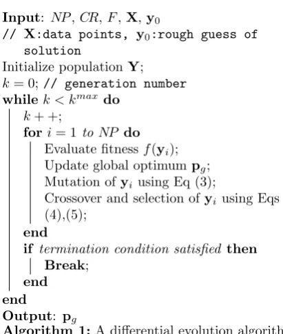
The pseudocode for optimization program is shown in Algorithm 1.

Input: NP,CR,F,X,y0

// X:data points, y0:rough guess of solution

Initialize populationY; k= 0; // generation number

whilek < kmax_do

k+ +;

fori= 1 toNP do

Evaluate fitnessf(yi);

Update global optimumpg;

Mutation ofyi using Eq (3);

Crossover and selection ofyi using Eqs

(4),(5);

end

if termination condition satisfied then Break;

end end

Output: pg

Algorithm 1:A differential evolution algorithm

The optimal configuration, i.e. the values of the pop-ulation size NP, the scaling factor F and the crossover rate CR, is very problem-dependent. According to the ’No-free-lunch theorems’, it is not possible to make the optimization program widely applicable whilst maintain-ing the best performance at every situation[5]. To obtain relatively good performance in different cases, the optimal parameter configuration is particularly obtained for each situation. Here meta-optimization is performed off-line us-ing the Local Unimodal Samplus-ing [6]. The runnus-ing speed of this algorithm is determined by the number of fitness

evaluations. Here this number is set no greater than 20 000. The unknown variables are the five motion parame-ters (Rotation about xand y axes and translation along x, y and z directions), the radius R, the conic constant k and polynomial coefficients{Ai} (if applicable). When

the shape parameters are all given, and only the optimiza-tion posioptimiza-tion of the measured data is to be calculated, this becomes the localization problem, and the dimension will be 5. The recommended parameter settings for different dimensions are listed in Table 1,

Table 1: Parameter settings of DE to aspherics

D NP CR F

5 23 0.866 0.7549 7 29 0.8745 0.7470 8 33 0.8884 0.7347 9 41 0.9046 0.7223 10 45 0.9148 0.7153 11 49 0.925 0.7087 12 52 0.9331 0.6972 13 55 0.9412 0.6808 14 57 0.9542 0.672 15 59 0.9636 0.6631 16 61 0.9729 0.6556

To prevent a too fast decrease of population diversity, the parameters need to satisfy the condition 2F2−2/NP+ CR/NP ≥0 [7]. Evidently it holds true for all the param-eters given here.

3. Improving the computational efficiency

This optimization problem is highly nonlinear and lots of local minima exist. To get better results form the DE optimization, the space of the unknown variables is nar-rowed by supplying a good initial guess for the solution. The orthogonal least squares[8] method is used for this purpose.

3.1. Calculating the orthogonal distances

It is straightforward to write the function of an aspheric surface asg(x) = 0 with x being a point on the surface. Normally the projection pointqassociated with the point

pis obtained from

{

g(q) = 0

∇g(q)×(p−q) = 0 (6)

using the Gauss-Newton or Levenberg-Marquardt algo-rithm.

But this method is time consuming, especially when there are many data points. Consequently at the first tens of iterations of the optimization program, the distance is approximated with [9]

d=±∥p− ∥q∥∥ ≈ g(p)

∥∇g(p)∥ (7)

As the motion and shape parameters have been approx-imately identified using linear least squares, the distance d will not be very large, i.e. p is reasonably near to the associated surface. Thus this approximation is acceptable. At the final iterations, the orthogonal distance is in turn calculated from Equation (6).

3.2. Reducing the number of data points

In practice, the number of measured data points may be up to millions, but actually only dozens of points de-termine the width of the error band (the point number is related with the number of unknown variables). If remov-ing some ’unnecessary’ points from the data set,the opti-mization process can be greatly accelerated. Fortunately, the alpha-shape technique meets this requirement.

Anα−shape is a well-defined polytope, derived from the Delaunay triangulation of the point set, with a param-eter α∈ Rcontrolling the desired level of detail [10]. In order to improve the discrepancy, we replace the z coor-dinates of the data points by the signed residuals resulted from the least squares fitting and then scale the points into a unit cubic. If implementing the 3D Delaunay triangula-tion, i.e. organizing the discrete points into a set of hedra, the real ’key points’ are likely located at some hedra with large circumscribed spheres, thus some tetra-hedra with small circumscribed spheres can be omitted. But many ’boundary points’ will be retained unnecessarily, hence the boundary and interior points are handled sepa-rately. Viewing from the z direction, the boundary points are recognized using the modified Graham scan method [11]. In the programme, the tetrahedra are sorted by their radii of circumscribed spheres (in descending order). The set for the points to be kept is initialized as null, and then the vertices of each tetrahedron are checked successively. The checking procedure is presented in Algorithm 2

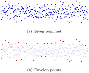
Figure 1 shows a 2D example. Given 300 points, 30 points on the envelop are sampled using the α− shape technique. The number of points to be retained is directly

(a) Given point set

(b) Envelop points

Figure 1: Point reduction usingα−shapes

related with the number of unknown variables. For exam-ple, in the evaluation of flatness (resp. sphericity), there

Input: point set{xi}Ni=1, points to be retained Y= Ø, Delaunay tetrahedraT∈NM×4_;

Find the boundary pointsB;

forj= 1 toM do fori= 1to4 do

if Tji∈B then

if Tji has the greatest positivez

coordinate or the smallest negativez coordinate among the four vertices ofTj

then

Put Tji intoY;

end else

Put Tji intoY;

end end

if The number of points in Ysatisfies the pre-set limit then

Break;

end end

Output: Y;

Algorithm 2: The checking process for the vertices to be retained

are three (resp. four) variables and four (resp. five) ex-treme points are needed to calculate the minimum zone error. For the same reason, ifnpolynomial terms are in-volved in the aspheric function, at leastn+ 8 points are needed. To avoid removing extreme points by mistake, 2n+ 14 points will be kept in the DE optimization.

4. Experimental validation and discussion

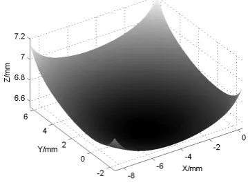
The validity of the proposed algorithm is verified with a data set of 8100 points, as shown in Figure 2. The unit of length here is mm if not specified otherwise. The nominal shape parameters are given as R = 520, k = −0.7, A4 =

5.2e−5, A6=−6.5e−6, A8= 3.11e−8, A10= 3.222e−9.

Noise with its amplitude ofσ= 0.98µmis introduced with the fractal Brownian function[12]. The dimensionality of the optimization problem is 11 and the control parameters in the DE program is adopted asNP = 49, CR= 0.929 and F = 0.74, in accordance with Table 1.

Figure 2: An aspheric surface

Table 2: Fitted results of the aspheric surface

method ODF DE withα DE withoutα

max min max min

PV/µm 3.79 3.29 3.21 3.31 3.21 time/s 0.15 5.10 4.34 115.02 126.85

of much longer running time. But the average time for the whole fitting process is less than five seconds, which is acceptable in practical applications. The point reduction technique using α− shapes reduced the running by 96%. It is worth noting that obtained PV form error has not been influenced by theα−shape point reduction, which is an essential requirement to that manipulation.

5. Conclusions

This paper proposes an optimization method using dif-ferential evolution to evaluate the peak-to-valley form er-rors of aspheric surfaces. To make the optimization pro-gram specifically works well for different dimensions of un-known variables, the parameter configuration is obtained using meta-optimization. Additionally, the alpha shapes is adopted to get the ’envelop points’ which potentially deter-mine the PV form error, so that the points involved in the optimization program are reduced. Experimental results prove the running time can be reduced by 96% without influencing the optimization results. This program can be utilized in aspheric surface fitting to calculate the shape parameters from the given measured data points or sur-face matching to determine the optimal relative position between the measured data and the nominal surface.

References

[1] ISO 10110-12 Optics and Photonics-Preparation of Drawings for Optical Elements and Systems-Part 12: Aspheric Surfaces, 2007.

[2] ISO 10110-5 Optics and Photonics-Preparation of Drawings for Optical Elements and Systems-Part 5:Surface Form Tolerances, 2007.

[3] K. Price, R. Storn, Differential evolution− a simple and ef-ficient adaptive scheme for global optimization over continu-ous spaces, Technical Report, Intern. Computer Science Inst., Berkley, 1995.

[4] A. K. Qin, P. N. Suganthan, Self-adaptive differential evolution algorithm for numerical optimization, in: 2005 IEEE Congress on Evolutionary Computation, volume 2, IEEE, IEEE Press, 2005, pp. 1785–91.

[5] D. H. Wolpert, W. G. Macready, No free lunch theorems for optimization, IEEE Trans. Evol. Comput 1 (1997) 67–82. [6] M. E. H. Pedersen, Tuning and Simplifying Heuristical

Opti-mization, Ph.D. thesis, University of Southampton, UK, 2010. [7] D. Zaharie, Critical values for the control parameters of

differ-ential evolution algorithms, in: R. Matouˇsk, P. Oˇsmera (Eds.), Proc. 8th Intern. Conf. Soft Computing Mendel, Brno, Czech Republic, pp. 62–7.

[8] X. Zhang, Freeform Surface Fitting for Precision Coordinate Metrology, Ph.D. thesis, University of Huddersfield, Hudders-field, UK, 2009.

[9] G. Taubin, Estimation of planar curves, surfaces and nonplanar spaces curves defined by implicit equations with applications to edge and range image segmentation, IEEE Trans. Patt. Anal. Mach. Intell. 13 (1991) 1115–38.

[10] H. Edelsbrunner, E. P. M¨ucke, Three-dimensional alpha shapes, ACM Trans. on Graphics 13 (1994) 43–72.

[11] X. Zhang, X. Jiang, P. J. Scott, Orthogonal distance fitting of precision free-form surfaces based onl1 norm, in: F. Pavese,

M. B¨ar, A. B. Forbes, et al. (Eds.), Adv. Math. and Comput. Tools in Metrology and Testing VIII, World Scientific, 2008, pp. 385–90.

[12] B. B. Mandelbrot, J. W. van Ness, Fractional brownian motions, fractional noises and applications, SIAM Review 10 (1968) 422– 37.