Sensitivity analysis for a 4 sensor probe used for bubble velocity vector measurement

Sensitivity analysis for a 4­sensor probe used for bubble velocity vector measurement

Original Citation

Pradhan, Suman, Lucas, Gary and Panayotopoulos, Nikolaos (2006) Sensitivity analysis for a 4­

sensor probe used for bubble velocity vector measurement. In: Proceedings of Computing and 

Engineering Annual Researchers' Conference 2006: CEARC’06. University of Huddersfield, 

Huddersfield, pp. 1­6. 

This version is available at http://eprints.hud.ac.uk/id/eprint/3806/

The University Repository is a digital collection of the research output of the

University, available on Open Access. Copyright and Moral Rights for the items

on this site are retained by the individual author and/or other copyright owners.

Users may access full items free of charge; copies of full text items generally

can be reproduced, displayed or performed and given to third parties in any

format or medium for personal research or study, educational or not­for­profit

purposes without prior permission or charge, provided:

•

The authors, title and full bibliographic details is credited in any copy;

•

A hyperlink and/or URL is included for the original metadata page; and

•

The content is not changed in any way.

For more information, including our policy and submission procedure, please

contact the Repository Team at: [email protected].

Sensitivity Analysis for a 4-Sensor Probe Used for Bubble Velocity

Vector Measurement

S. Pradhan, G. Lucas and N. Panayotopoulos

University Of Huddersfield

Abstract

In recent years, there has been an increase in the level of interest shown in making flow rate measurements in multiphase flow. This in part has been brought about by the metering requirements of the oil and natural gas industries. Measuring the volumetric flow rate of each of the flowing components is often required and this is particularly true in production logging applications, where it may be necessary to measure the flow rates of oil and water down hole in vertical and inclined oil wells. Within the University of Huddersfield [1], work has been undertaken on the study of vertical and inclined multiphase flow. Previous work was based on the use of local, dual-sensor conductance probes to obtain the local axial velocity and volume fraction of the bubbles in multiphase flows [1]. The purpose of this research presented in this paper is to investigate the sensitivity of 4-sensor-probes, used for bubble velocity vector measurement to dimensional measurement errors of the probe and to errors in measuring the time intervals between the surfaces of the bubble contacting the sensors in the probe.

The probe was manufactured from 0.3mm diameter stainless steel acupuncture needles due to their high level of rigidity. The acupuncture needles were mounted inside a stainless steel tube with an

outer diameter of 4mm [2]. A procedure was carried out whereby an error on a specific probe

dimension was introduced (errors in the range of -10 % to +10% of the true value of the dimension were used). The error in the measured bubble velocity vector was then investigated. A similar

procedure was used to investigate the effect of measurement errors in the probe ‘time intervals’

δ

t

₁₁,

22

t

δ

and

δ

t

₃₃ on the measured bubble velocity vector. NB:The bubble velocity vector is quantified in

terms of a polar angle

α

an azimuthal angle

β

and a velocity magnitude

v

.

Results demonstrate that it is crucial to measure probe dimensions precisely (within the range of ±1%) as small errors in the probe dimensions or measured time intervals can give rise to large errors in the values of

α

,

β

and

v

.

Nomenclature

α

Polar angle (degrees)

β

azimuthal angle (degrees)

v

Velocity magnitude (m/s)

11

t

δ

δ

t

₂₂

δ

t

₃₃ Time delays (s) calculated from the times at which the bubble surface contacts

sensors 0, 1, 2 and 3 [3].

1 INTRODUCTION

As a part of a previous research project within the University of Huddersfield many dual and four sensor probes were built to measure the flow velocity of the bubbles in multiphase flow. This has relevance to many applications e.g. the oil industries, chemical industries and mines. [4]

The purpose of this research is based on the extensive research on sensitivity of 4 sensor-probes that were being used to measure the properties of multiphase flow. To be specific these properties relates to local and mean velocity and local velocity vector of disperse phase.

As these probes were being used in multiphase flow measurement it will be wise to describe the different types of multiphase flow that can exist:-

Basically there are two types of flows:-

Understanding of these types of flow requires complex physics. Several combinations of flowing substances can be considered as multiphase flow e.g. gas-liquid flows, liquid-liquid flows, liquid-solids flows, gas-solids flows, and gas-liquid-solids flows etc.

According to its flow structure and pattern, a vertical multiphase flow can be generalized into four major different types known as bubbly flow, slug flow; churn flow and the annular flow (see Figure 1). The flow structure depends on the flow rates of the flowing components e.g. continuous water and dispersed oil or air in case of the experiments carried out within the University.

Generalising the flow pattern as in figure 1, the flow that contains a large amount of water comparing to that of disperse phase is categorised as bubbly flow. It contains numerous bubbles (of various size) flowing through out the pipeline.

Gas-liquid flows containing greater amount of disperse phase then in bubbly flow are characterised by the gas flowing with a bullet shape (or Taylor Bubble). In this type of flow a few bubbles can be seen flowing in between of these bullet shaped bubbles.

Churn flow can be identified with the presence of irregular or chaotic movement of the dispersed phase, that occupying almost all the parts of pipe. Similar to a slug flow these flow also being separated by numerous of bubbly flow in between irregular shaped flow.

With high rate of dispersed phase flow, allowing water to flow only with thin layer along side the wall is described as an annular flow.

The multiphase flows described above are commonly encountered in the oil, gas, chemical and mining industries and in nuclear plants.

2 CONDUCTIVITY PROBE MANUFACTURE AND STRUCTURE

Background

Local measurement techniques for multiphase flow can be categorized as intrusive or non-intrusive methods.

1. Intrusive method include:

Conductivity probes using needles, heat transfer probes, hot wire anemometers

In these methods any of the above probes were inserted into the systems to get results.

2. Non intrusive method

Methods where local flow properties can be measured where the equipment is not inserted into the system include:

Light attenuation, electrical resistance tomography (ERT), photography and image analysis, laser Doppler anemometry and phase Doppler anemometry

Within the University of Huddersfield local flow property measurements are carried out as an intrusive method using an intrusive, four-sensor conductivity probe. The probe was manufactured from 0.3mm diameter stainless steel acupuncture needles due to their high level of rigidity. The acupuncture

needles were mounted inside a stainless steel tube with an outer diameter of 4mm [2] as shown in

figure 2. Both the local velocity vector profile and local volume fraction profile of the dispersed phase

can be obtained from the four-sensor probe [2].

One of the important aspects of the current research is to minimize the bubble-probe interaction so that the effect of the probe on the bubble velocity vector is as small as possible. Therefore an important factor that one must kept in mind while fabricating probe is to make them as small as possible in terms of dimensions. This has an additional benefit since the measurement accuracy is improved with smaller probes due to the fact that there is a higher possibility for the bubble to strike twice in each of the four sensors within the probe – as required by the measurement technique.

With the smaller probe it will be possible to measure the higher range of polar angles for which the bubble’s velocity can be measured. From the studies carried out by R. Mishra, when the separation of

the sensors is 1mm the minimum polar angle α [fig 2 shows angle definition] is about 270. This means

that for flows where the droplets have 5mm diameter will strike each rear sensor twice when γ=270. In

case where the separation of the sensors is 0.5mm, the value of γ has increased to about 450. It can

3 Theories

With the help of a local four-sensor probe we can measure various characteristics of the dispersed phase including the local volume fraction and the local vector velocity individual bubble. The bubble

velocity vector is expressed in terms of the velocity magnitude

v

and the velocity direction, which in

turn can be expressed in terms of a polar angle

α

and an azimuthal angle

β

. Based on the

assumptions given in [1] a mathematical model was introduced [3] to calculate

α

,

β

and

v

, for a

given bubble, from the time intervals

δ

t

₁₁,

δ

t

₂₂ and

δ

t

₃₃ calculated from measurements of the times at which each of the four sensors came into contact with the surface of the bubble.

In the work presented in this paper

α

,

β

and

v

are assumed to be known along with the probe

dimensions

x

_i

,

y

_i

and

z

_i (where i = 1, 2 and 3) allowing

δ

t

₁₁,

δ

t

₂₂ and

δ

t

₃₃to be calculated from equations 1, 2 and 3 below.

2

cos

cos

sin

sin

sin

11 1 1 1

dt

z

y

x

α

β

+

α

β

+

α

=

υ

(1)

2

cos

cos

sin

sin

sin

22 2 2 2

dt

z

y

x

α

β

+

α

β

+

α

=

υ

(2)

2

cos

cos

sin

sin

sin

33 3 3 3

dt

z

y

x

α

β

+

α

β

+

α

=

υ

(3)

Errors are then introduced into either the probe dimensions

x

_i

,

y

_i

and

z

_i or into the time delays

δ

t

₁₁,

22

t

δ

and

δ

t

₃₃ and new, estimated values of

β

’ and

α

’ are calculated from equations 4 and 5 below

from these incorrect probe dimensions or time delays.













−













−

−













−













−













−













−

−













−













−

=

33 3 11 1 22 2 11 1 22 2 11 1 33 3 11 1 22 2 11 1 33 3 11 1 33 3 11 1 22 2 11 1

'

tan

t

x

t

x

t

z

t

z

t

x

t

x

t

z

t

z

t

y

t

y

t

z

t

z

t

y

t

y

t

z

t

z

δ

δ

δ

δ

δ

δ

δ

δ

δ

δ

δ

δ

δ

δ

δ

δ

β

(4)

'

cos

'

sin

'

tan

22 2 11 1 22 2 11 1 11 1 22 2

β

δ

δ

β

δ

δ

δ

δ

α













−

+













−













−

=

t

y

t

y

t

x

t

x

t

z

t

z

(5)

Finally an estimated value

v

’ of the velocity magnitude can be calculated by substituting

β

’ and

α

’ into any of equations 1 to 3.

The purpose of the investigation was to determine the influence of the errors in

δ

t

_ii and

i i

i

y

z

x

,

and

(i=1 to 3) on the size of the errors in

β

’,

α

’ and

v

’.

4 RESULTS OF SENSITIVITY ANALYSIS

A series of experiments were performed to measure the sensitivity of local-four sensor probe for air-in-water flows. The measurements were carried out at mentioned true values by introducing an error

at different measures of the probe dimension

x

_i

,

y

_i

and

z

_iand their combinations. The measurement

was also calculated using time delays

δ

t

_ii with the newly made probe (measurement shown in table

4.1 Analysis of data with error at

z1

with true value

of

α

= 0.1°,

β

= 0.001° and

v

=0.25m/s

Figure 3 shows the calculated values of

β

’

,

α

’

and

v

’

for the data mentioned above

From the

figure it can be seen with an error -2.5% of z1 the polar angle increased from 1.0° to 1.64969118° and

velocity increased from 0.25m/s to 0.259036143 m/s .

4.2 Analysis of data with error at

z1

z2 with true value

of

α

= 0.1°,

β

= 0.001° and

v

=0.25m/s

Next the error was introduced in z1 and z2 in the same original measure as in table 1. As mentioned

above the

β

’

,

α

’

and

v

’was calculated again to check any new error which is presented in figure 4.

From where it can be seen that at same error 2.5% of z1 the polar angle changed from 1.0° to

-1.031701° and velocity increased from 0.25m/s to 0.2510185 m/s .

From the above two results it is concluded that with the error in 2 components z1 z2 or z3 the range of error is lesser then that of when the error was only in one components. That is due to the fact

equation 4 and 5 contained all the variables

cancelling

the error. From the result it is also noticed

that even with small error as little as

±

2.5% (which is not much when it comes to micron) causes a

variation of angle

α

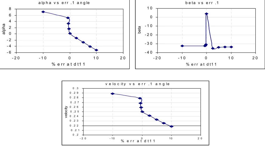
from 0.1° to 1.65°. Therefore it is vital to reduce an error to get accurate results.

4.3 Analysis of data with error at dt

11 with true value of

α

= 0.1

0

°

and 5

°,

β

=

4

°

and

v

=0.25m/s

Realising the possibilities of making error while taking reading of

δ

t

₁₁,

δ

t

₂₂and

δ

t

₃₃. Detail analysis

had been carried out introducing an error in

δ

t

₁₁ of the same range of ±10% in an angle of 0.1° and

5°. Figure 5 and 6 shows the results of

β

’

,

α

’

and

v

’ at an angle of 0.1° and 5° respectively. From the results it can be seen that there is not much difference in terms of velocity where as the angle give a dramatic change from 0.1° to 1.6° and 5° to 6.4° from which it is possible to say that the higher the polar angle the lesser the effect of errors but the fact cannot be ignored that the possibilities of making error and variation of

α

due to error in

δ

t

₁₁.

5 CONCLUSIONS

From the results we can conclude that even a micron difference in the measurement in dimensions

(which is visibly impossible to figure out) makes a huge difference in the data output in terms of’

,

α

β

and

v

. Due to the size of needles, it is possible to make an error in many ways among which that

are listed below.

• Taking measurement: - Major possibility of making error is while taking the measurement of

needles as errors are in microns which are virtually impossible to figure out with naked eye. Also with the way that the probes were built and measuring process, it is only possible to focus either rare or the front sensor, showing the possibility of making errors.

• While taking readings: - there is a high possibility of an unexpected result due to the size of the

probe itself. Higher the dimension, higher the possibility in alteration of bubble structure and characteristics.

REFERENCES

1

Mishra R., Lucas G. P., Kieckhoefer H., “A model for obtaining the velocity vectors of spherical droplets in multiphase flows from measurements using an orthogonal four-sensor probe.”, Meas. Sci. Technol.m volume 13, pages 1488-1498, 2002

2 G.P.Lucas, N Panayotopoulos “Power law approximation to gas volume fraction and velocity profile in low void fraction vertical gas-liquid flows”

3 G. P. Lucas, R. Mishra “Measurement of bubble velocity components in a swirling gas-liquid pipe flow using a local four sensor conductance probe.”

Figure 1:- Types of multiphase flow Fig 2 showing angle projecting with respect to bubble flow

Figure3: variation

α

,

β

and

v

of error at z1 (true value of

α

= 0.1°,

β

=0.001 and

v

=0.25m/s)

Figure4: variation

α

,

β

and

v

of error at z1 & z2 (true value of

α

= 0.1°,

β

=0.001 and

v

=0.25m/s)

V

x z

V

y α

β

Dotted line is projection of V onto xy plane 1

0

Axis of probe holder aligned with pipe axis

2 3

a lp h a v s % e r r o n z 1 a n d z 2

- 5 - 4 - 3 - 2 - 1 0 1 2 3 4 5

- 1 5 - 1 0 - 5 0 5 1 0 1 5

% e r r o n z 1 a n d z 2

al

ph

a

beta vs % err on z1 and z2

-10 0 10 20 30 40 50 60

-15 -10 -5 0 5 10 15

% err on z1 and z2

bet

a

v e l v s % e r r o n z 1 a n d z 2

0 . 2 4 0 . 2 5 0 . 2 5 0 . 2 5 0 . 2 5 0 . 2 5

- 1 5 - 1 0 - 5 0 5 1 0 1 5

% e r r o n z 1 a n d z 2

ve

l

a lp h a v s % e r r in z 1

- 6 - 4 - 2 0 2 4 6 8

- 1 5 - 1 0 - 5 _{% e r r in z 1}0 5 1 0 1 5

al

ph

a

beta v s % err in z 1

-40 -30 -20 -10 0 10

-15 -10 -5 0 5 10 15

% err in z 1

be

ta

v el v s % err in z 1

0.20 0.22 0.24 0.26 0.28 0.30 0.32

-15 -10 -5 0 5 10 15

% err in z 1

ve

[image:7.595.69.493.92.327.2] [image:7.595.65.500.360.633.2]

Figure 5: variation

α

,

β

and

v

of error at dt11 (true value of

α

= 0.1°,

β

=4 and

v

=0.25m/s)

Figure 6: variation

α

,

β

and

v

of error at dt11 (true value of

α

= 5°,

β

=4 and

v

=0.25m/s)

4s1/4s4 X (mm) Y(mm) Z(mm)

Sensor 1 0.7889 (x1) 0.106 (y1) 1.1778 (z1)

Sensor 2 0.0556 (x2) 0.183(y2) 1.1223(z2)

Sensor 3 -1.122 (x3) 0.096(y3) 1.0556(z3)

Table 1. Measured dimensions of the 4s1/4s4 4-sensor probes.

alpha vs err at 5 deg

-5 0 5 10 15

-15 -10 -5 0 5 10 15

%err at dt11

al

ph

a

beta vs err at 5 deg

-120 -80 -40 0 40 80 120

-15 -10 -5 0 5 10 15

% err at dt11

be

ta

v el v s err at 5 deg

0.2 0.22 0.24 0.26 0.28 0.3

-15 -10 -5 0 5 10 15

% err at dt11

ve

lo

ci

ty

a lp h a v s e r r . 1 a n g le

- 6 - 4 - 2 0 2 4 6 8

- 2 0 - 1 0 0 1 0 2 0

% e r r a t d t1 1

alp

h

a

b e t a v s e r r . 1

- 4 0 - 3 0 - 2 0 - 1 0 0 1 0

- 2 0 - 1 0 0 1 0 2 0

% e r r a t d t 1 1

bet

a

v e lo c it y v s e r r . 1 a n g le

0 . 2 0 . 2 1 0 . 2 2 0 . 2 3 0 . 2 4 0 . 2 5 0 . 2 6 0 . 2 7 0 . 2 8 0 . 2 9 0 . 3

- 2 0 - 1 0 0 1 0 2 0

% e r r a t d t 1 1

ve

lo

ci

[image:7.595.70.498.670.713.2]