Three essays on time series: spatio temporal modelling, dimension reduction and change point detection

The London School of Economics and Political Science

Three Essays on Time Series: Spatio-Temporal Modelling,

Dimension Reduction and Change-Point Detection

Baojun Dou

Supervisor: Prof. Qiwei Yao

A thesis submitted to the Department of Statistics of the London School of Economics for

Declaration

I certify that the thesis I have presented for examination for the PhD degree of the London School of Economics and Political Science is solely my own work other than where I have clearly indicated that it is the work of others (in which case the extent of any work carried out jointly by me and any other person is clearly identified in it). I confirm that Section 1.5 was jointly co-authored with Dr. Maria Lucia Parrell from University of Salerno, Italy and Section 3.2 was jointly co-authored with Prof. Rongmao Zhang from Zhejiang University, China.

Abstract

Modelling high dimensional time series and non-stationary time series are two import as-pects in time series analysis nowadays. The main objective of this thesis is to deal with these two problems. The first two parts deal with high dimensionality and the third part considers a change point detection problem.

In the first part, we consider a class of spatio-temporal models which extend popular econometric spatial autoregressive panel data models by allowing the scalar coefficients for each location (or panel) different from each other. The model is of the following form:

yt =D(λ0)Wyt+D(λ1)yt−1+D(λ2)Wyt−1+εt, (1)

whereyt= (y1,t, . . . , yp,t)T represents the observations fromplocations at timet,D(λk) = diag(λk1, . . . , λkp) andλkjis the unknown coefficient parameter for thej-th location, andW is thep×pspatial weight matrix which measures the dependence among different locations. All the elements on the main diagonal of W are zero. It is a common practice in spatial econometrics to assume W known. For example, we may let wij = 1/(1 +dij), for i ̸=j, where dij ≥ 0 is an appropriate distance between the i-th and the j-th location. It can simply be the geographical distance between the two locations or the distance reflecting the correlation or association between the variables at the two locations. In the above model, D(λ0) captures the pure spatial effect, D(λ1) captures the pure dynamic effect,

and D(λ2) captures the time-lagged spatial effect. We also assume that the error term

εt = (ε1,t, ε2,t, . . . , εp,t)T in (1) satisfies the condition Cov (yt−1,εt) = 0. When λk1 =· · ·=

(1) contains 3p unknown parameters. To overcome the innate endogeneity, we propose a generalized Yule-Walker estimation method which applies the least squares estimation to a Yule-Walker equation. The asymptotic theory is developed under the setting that both the sample size and the number of locations (or panels) tend to infinity under a general setting for stationary and α-mixing processes, which includes spatial autoregressive panel data models driven by i.i.d. innovations as special cases. The proposed methods are illustrated using both simulated and real data.

In part 2, we consider a multivariate time series model which decomposes a vector process into a latent factor process and a white noise process. Let yt = (y1,t,· · · , yp,t)T be an observable p×1 vector time series process. The factor model decomposes yt in the following form:

yt =Axt+εt, (2)

sample size and the dimensionality tend to infinity. When the common factor is weak in the sense that δ > 1/2 in Lam, Yao and Bathia (2011)’s paper, the new sparse estimator may have a faster convergence rate. Numerically, we employ the generalized deflation method (Mackey (2009)) and the GSLDA method (Moghaddam et al. (2006)) to approximate the estimator. The tuning parameter is chosen by cross validation. The proposed method is illustrated with both simulated and real data examples.

The third part is a change point detection problem. we consider the following covariance structural break detection problem:

Cov(yt)I(tj₋1 ≤t < tj) =Σtj−1, j = 1,· · · , m+ 1,

where yt is a p×1 vector time series, Σtj−1 ≠ Σtj and {t1, . . ., tm} are change points,

1 =t0 < t1 <· · ·< tm+1 =n. In the literature, the number of change points m is usually

assumed to be known and small, because a large m would involve a huge amount of com-putational burden for parameters estimation. By reformulating the problem in a variable selection context, the group least absolute shrinkage and selection operator (LASSO) is proposed to estimate m and the locations of the change points {t1, . . ., tm}. Our method

is model free, it can be extensively applied to multivariate time series, such as GARCH and stochastic volatility models. It is shown that both m and the locations of the change points {t1, . . . , tm} can be consistently estimated from the data, and the computation can

Acknowledgments

I would like to express my deepest gratitude and utmost respect to my supervisor Professor Qiwei Yao. His continued guidance, encouragement and tremendous support leads me to the completion of this work during my four years PhD and one year MSc study. He is not only a supervisor of my research but also of my life. It is my great honor in my life to be his student.

I would also like to thank my second supervisor, Dr. Clifford Lam, who helped me a lot and answered me a lot of tedious and time consuming technique problems in the literatures. I am grateful to Professor Oliver Linton and Dr. Barigozzi Matteo for willingly accepting to be part of the examination committee and to evaluate this thesis.

Contents

Chapter 1: Generalized Yule-Walker Estimation for Spatio-Temporal

Mod-els with Unknown Diagonal Coefficients 9

1.1 Introduction . . . 9

1.2 Model and Estimation Method . . . 11

1.2.1 Models . . . 11

1.2.2 Generalized Yule-Walker estimation . . . 12

1.2.3 A root-n consistent estimator for largep . . . 14

1.3 Theoretical properties . . . 16

1.3.1 Asymptotics for fixed p . . . 18

1.3.2 Asymptotics with diverging p . . . 19

1.4 Simulation study . . . 24

1.4.1 Scenario 1 . . . 24

1.4.2 Scenario 2 . . . 26

1.5 Real data analysis . . . 28

1.5.1 European Consumer Price Indices . . . 28

1.5.2 Modeling mortality rates . . . 34

1.7 Appendix: Proofs . . . 37

Chapter 2: Sparse Factor Modelling for Vast Time Series 50 2.1 Introduction . . . 50

2.2 Model and Estimation Method . . . 52

2.2.1 Models . . . 52

2.2.2 Estimation . . . 55

2.3 Theoretical Properties . . . 57

2.4 Choice of Tuning Parameter . . . 60

2.5 Simulation Studies . . . 61

2.5.1 scenario 1 . . . 61

2.5.2 scenario 2 . . . 62

2.5.3 scenario 3 . . . 64

2.5.4 Cross Validation . . . 65

2.6 Real Data Analysis . . . 67

2.7 Appendix: Proofs . . . 69

Chapter 3: Group Lasso for Covariance Matrix Break Detection 79 3.1 Introduction . . . 79

3.2 Problem and Estimation Method . . . 81

3.2.1 Problem . . . 81

3.2.2 One-step Estimation . . . 81

3.2.3 Two-step estimation procedure . . . 83

3.4 Simulation Studies . . . 87

3.4.1 Scenario 1 . . . 88

3.4.2 Scenario 2 . . . 89

3.4.3 Scenario 3 . . . 90

3.5 Future work . . . 91

3.6 Appendix: Proofs . . . 91

Chapter 4: Two Simple Results 101 4.1 An extension of Bickel, P.J. and Levina, E (2008)’s result . . . 101

Chapter 1: Generalized Yule-Walker

Estimation for Spatio-Temporal

Models with Unknown Diagonal

Coefficients

1.1

Introduction

are more efficient than the QML estimation (Lee, 2001). Lee and Yu (2010a) classifies SDPD models into three categories: stable, spatial cointegration and explosive cases. As pointed out by Bai and Shi (2011), the cases with a large number of cross sectional units and a long history are rare. Hence it is pertinent to consider the setting with short time spans in order to include as many locations as possible. Both estimation method and asymptotic analysis need to be adapted under this new setting. Yu et al. (2008) and Yu et al. (2012) investigate the asymptotic properties when both the number of locations and the length of time series tend to infinity for both the stable case and spatial cointegration case, and show that QMLE is consistent.

(2012). We develop the asymptotic properties under a general setting for stationary and α-mixing processes, which includes the spatial autoregressive panel data models driven by i.i.d. innovations as special cases.

The rest of the paper is organized as follows. Section 1.2 introduces the new model, its motivation and the generalized Yule-Walker estimation method. The asymptotic theory for the proposed estimation method is presented in Section 1.3. Simulation results and real data analysis are reported, respectively, in Section 1.4 and 1.5. All the technical proofs are relegated to an Appendix.

1.2

Model and Estimation Method

1.2.1

Models

The model considered in this paper is of the following form:

yt =D(λ0)Wyt+D(λ1)yt−1+D(λ2)Wyt−1+εt, (1.2.1)

and D(λ2) captures the time-lagged spatial effect. We also assume that the error term

εt = (ε1,t, ε2,t, . . . , εp,t)T in (1.2.1) satisfies the condition Cov (yt−1,εt) = 0. When λk1 =

· · · = λkp for k = 0,1,2, (1.2.1) reduces to the model of Yu et al. (2008), in which there are only 3 unknown regressive coefficient parameters. In general the regression function in (1.2.1) contains 3p unknown parameters.

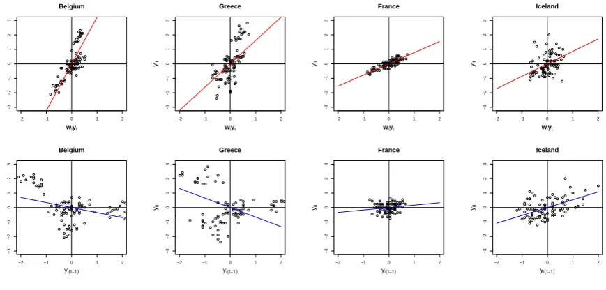
The extension to use different scalar coefficients for different locations is motivated by practical needs. For example, we analyze the monthly change rates of the consumer price index (CPI) for the EU member states over the years 2003-2010. The detailed analysis for this data set will be presented in section 1.5. Figure 1.1 presents the scatter-plots of the observed data yi,t versus the spatial regressor wTi yt and yi,t−1, for some of the EU

member states, where wT

i is the i-th row vector of the weight matrix W which is taken as the sample correlation matrix with all the elements on the main diagonal set to be 0. The superimposed straight lines are the simple regression lines estimated using the newly proposed method in Section 2.2 below. It is clear from Figure 1.1 that at least Greece and Belgium should have a different slope from those of France or Iceland.

1.2.2

Generalized Yule-Walker estimation

As yt occurs on both sides of (1.2.1), Wyt and εt are correlated with each other. Apply-ing least squares method directly based on regressApply-ing yt on (Wyt,yt−1,Wyt−1) leads to

−2 −1 0 1 2 −3 −2 −1 0 1 2 3 Belgium

wiyt

yit

−2 −1 0 1 2

−3 −2 −1 0 1 2 3 Greece

wiyt

yit

−2 −1 0 1 2

−3 −2 −1 0 1 2 3 France

wiyt

yit

−2 −1 0 1 2

−3 −2 −1 0 1 2 3 Iceland

wiyt

yit

−2 −1 0 1 2

−3 −2 −1 0 1 2 3 Belgium

yi(t−1)

yit

−2 −1 0 1 2

−3 −2 −1 0 1 2 3 Greece

yi(t−1)

yit

−2 −1 0 1 2

−3 −2 −1 0 1 2 3 France

yi(t−1)

yit

−2 −1 0 1 2

−3 −2 −1 0 1 2 3 Iceland

yi(t−1)

yit

Figure 1.1: Plots of the monthly change ratesyi,t of CPI against the spatial regressorwTi yt (on the top) and the dynamic regressoryi,t₋1 (on the bottom) for four EU member states in

2003-2010. The superimposed straight lines were estimated by the newly proposed method in Section 2.2.

We propose below a new estimation method which applies the least squares method to each individual row of a Yule-Walker equation. To this end, letΣk= Cov(yt+k,yt) for any k ≥0. Note that we always assume that yt is stationary, see condition A2 and Remark 1 in Section 1.3 below. Then the Yule-Walker equation below follows from (1.2.1) directly.

(I−D(λ0)W)Σ1 = (D(λ1) +D(λ2)W)Σ0,

whereI is a p×p identity matrix. The i-th row of the above equation is

(eT_i −λ0iwTi )Σ1 = (λ1ieTi +λ2iwTi )Σ0, i= 1, . . . , p, (1.2.2)

matrices

b

Σ1 =

1 n

n−1

∑

t=1

yt+1ytT and Σb0 =

1 n

n

∑

t=1

ytyTt.

We estimate (λ0i, λ1i, λ2i)T by the least squares method, i.e. to solve the minimization problem

min λ0i,λ1i,λ2i

∥ΣbT₁(ei−λ0iwi)−Σb0(λ1iei+λ2iwi)∥22.

The resulting estimators are called generalized Yule-Walker estimators which admits the explicit expression:

(bλ0i,bλ1i,bλ2i)T = (XbiTXbi)−1XbTi Ybi, (1.2.3)

where

b

Xi = (Σb T

1wi,Σb0ei,Σb0wi) and Ybi =Σb T

1ei. More explicitly, b Xi = ( 1 n n ∑ t=1

yt₋1(wTi yt), 1 n

n

∑

t=1

yt₋1yi,t−1,

1 n

n

∑

t=1

yt₋1(wiTyt−1)

)

, Yib = 1 n

n

∑

t=1

yt₋1yi,t.

Then it holds that for i= 1,· · · , p,

        b

λ0i

b

λ1i

b

λ2i

        −        

λ0i λ1i λ2i

       

= (XbT_i Xbi)−1

        1 n ∑n

t=1y

T

t−1(wTi yt)× _n1

∑n

t=1εi,tyt−1 1

n

∑n

t=1yTt−1yi,t−1× _n1

∑n

t=1εi,tyt−1 1

n

∑n

t=1y

T

t−1(wiTyt−1)×_n1

∑n

t=1εi,tyt−1

        .

1.2.3

A root-

n

consistent estimator for large

p

equations increases. See, for example, a similar result in Theorem 1 of Chang, Chen and Chen (2015). A further compounding factor is that the estimation for the covariance matrices Σ0, Σ1 using their sample counterparts leads to non-negligible errors even when

n → ∞ (as long as p is very large). Below we propose an alternative estimator which restricts the number of the estimation equations to be used in order to restore the √ n-consistency and the asymptotic normality.

For i = 1,· · · , p, put Xi = (ΣT1wi,Σ0ei,Σ0wi). Note that the k-th row of Xi is (eT

kΣ T

1wi,

eT_kΣ0ei,eTkΣ0wi) which is the covariance between yk,t−1 and (wTi yt, yi,t−1, wiTyt−1). Let

ρ(_ki)=e_kTΣT₁wi+e_kTΣ0ei+eTkΣ0wi, k = 1,· · · , p. (1.2.4)

Thenρ(_ki)may be viewed as a measure for the correlation betweenyk,t−1and (wTi yt, yi,t−1,wTi yt−1)T.

When ρ(_ki) is small, say, close to 0, the k-th equation in (1.2.2) carries little information on (λ0i, λ1i, λ2i). Therefore as far as the estimation for (λ0i, λ1i, λ2i) is concerned, we only keep the k-th equation in (1.2.2) for large ρ(_ki).

Let zi_t−1 be the di ×1 vector consisting of those yk,t−1 corresponding to the di largest

b

ρ(_ki) (1≤k ≤p), where ρb_k(i) is defined as in (1.2.4) but with (Σ1, Σ0) replaced by (Σb1, Σb0).

The new estimator is defined as

(eλ0i, eλ1i, eλ2i)T = (ZbTi Zbi)−1ZbiTYei, i= 1,· · ·, p. (1.2.5) where

b

Zi =

(₁

n n

∑

t=1

zi_t−1(w_iTyt), 1 n

n

∑

t=1

zi_t−1yi,t₋1,

1 n

n

∑

t=1

zi_t−1(wT_i yt₋1)

)

, (1.2.6)

and

e

Yi = 1 n

n

∑

t=1

Now it holds that         e

λ0i

e

λ1i

e

λ2i

        −        

λ0i λ1i λ2i

       

= (ZbT_i Zbi)−1ZbTi

        1 n ∑n

t=1εi,tzit−1 1

n

∑n

t=1εi,tz

i t−1 1

n

∑n

t=1εi,tz

i t−1

        .

Theorem 3 in Section 3 below shows the asymptotic normality of the above estimator provided that the number of estimation equations used satisfies condition di =o(

√

n).

1.3

Theoretical properties

We introduce some notations first. For ap×1 vector v= (v1,· · · , vp)T,∥v∥2 =

√∑p

i=1vi2 is the Euclidean norm, ∥v∥1 =

∑p

i=1|vi| is the L1 norm. For a matrix H= (hij), ∥H∥F =

√

tr(HT_{H) is the Frobenius norm,} ∥_H∥

2 =

√

λmax(HTH) is the operator norm, where

λmax(·) is the largest eigenvalue of a matrix. We denote by |H|the matrix (|hij|) which is a matrix of the same size asH but with the (i, j)-th element hij replaced by|hij|. Note the determinant of H is denoted by det(H). A strictly stationary process {yt} is α-mixing if

α(k)≡ sup A∈F0

−∞,B∈Fk∞

P(A)P(B)−P(AB)→0, as k → ∞, (1.3.7)

where F_ij denotes the σ-algebra generated by {yt, i≤t ≤j}. See, e.g., Section 2.6 of Fan and Yao (2003) for a compact review of α-mixing processes.

Let S(λ0)≡I−D(λ0)W be invertible. It follows from (1.2.1) that

yt=Ayt−1+S−1(λ0)εt,

where A=S−1_(λ

0)(D(λ1) +D(λ2)W). Some regularity conditions are now in order.

A1. The spatial weight matrix W is known with zero main diagonal elements; S(λ0) is

A2. (a) The disturbance εt satisfies

Cov(yt−1,εt) = 0.

(b) The process {yt} in model (1.2.1) is strictly stationary and α-mixing with α(k), defined in (1.3.7), satisfying

∞ ∑

k=1

α(k)4+γγ _<∞_,

for some constant γ >0.

(c) For γ >0 specified in (b) above,

sup p

EwT_i Σ0yt

4+γ

<∞, sup p

EwT_i Σ1yt

4+γ

<∞, sup p

EeT_i Σ0yt

4+γ <∞, sup

p

Ew_iTyt

4+γ

<∞, sup p

EeT_i yt

4+γ <∞,

where wi denotes the i-th row of W. The diagonal elements of Vi defined in (1.3.8) are bounded uniformly inp.

A3. The rank of matrix (ΣT₁wi,Σ0ei,Σ0wi) is equal to 3.

B1. The errorsεi,t arei.i.dacrossiand twith E(εi,t) = 0, Var(εi,t) = σ20, and E|εi,t|

4+γ <

∞. The density function of εi,t exists.

B2. The row and column sums of |W| and |S−1(λ0)| are bounded uniformly in p.

B3. The row and column sums of ∑∞_j=0|Aj_{| are bounded uniformly inp.}

Now we are ready to present the asymptotic properties for (bλ0i,bλ1i,bλ2i)T, i= 1, . . . , p, with fixedp and n → ∞first, and then p→ ∞ and n → ∞.

1.3.1

Asymptotics for fixed

p

Fori= 1, . . . , p, let

Σy,εi(j) = Cov(yt−1+jεi,t+j,yt−1εi,t), j = 0,1,2,· · · ,

Σy,εi =Σy,εi(0) +

∞ ∑

j=1

[

Σy,εi(j) +Σ

T

y,εi(j)

]

,

Vi =

        wT

i Σ1ΣT1wi wiTΣ1Σ0ei wTi Σ1Σ0wi wT_i Σ1Σ0ei eTi Σ0Σ0ei eTi Σ0Σ0wi

wT

i Σ1Σ0wi eTi Σ0Σ0wi wTi Σ0Σ0wi

        , (1.3.8) and

Ui =

        wT

i Σ1Σy,εiΣ

T

1wi wTi Σ1Σy,εiΣ0ei w

T

i Σ1Σy,εiΣ0wi

wT

i Σ1Σy,εiΣ0ei e

T

i Σ0Σy,εiΣ0ei e

T

i Σ0Σy,εiΣ0wi

wTi Σ1Σy,εiΣ0wi e

T

i Σ0Σy,εiΣ0wi w

T

i Σ0Σy,εiΣ0wi

        . (1.3.9)

Theorem 1 Let conditions A1 – A3 hold and p ≥ 1 be fixed. Then as n → ∞, it holds that √ n                 b

λ0i

b

λ1i

b

λ2i

        −        

λ0i λ1i λ2i

                d −

where Vi and Ui are given in (1.3.8) and (1.3.9).

1.3.2

Asymptotics with diverging

p

When p diverges together with n, Ui,Vi in (1.3.9) and (1.3.8) are no longer constant matrices. Let U−

1 2

i be a matrix such that (U

−1 2

i )2 =U−

1

i .

Theorem 2 Let condition A1 – A3 hold.

(i) As n → ∞, p→ ∞ and p=o(√n),

√

nU−

1 2

i Vi

                b

λ0i

b

λ1i

b

λ2i

        −        

λ0i λ1i λ2i

                d −

→N(0,I3), i= 1, . . . , p.

(ii) As n → ∞, p→ ∞, √n=O(p) and p=o(n),

        b

λ0i

b

λ1i

b

λ2i

        −        

λ0i λ1i λ2i

        2

=Op

(_p

n

)

, i= 1, . . . , p.

Intuitively, condition A2(c) reflects the spatial dependence, that is the structures of Σ0

and Σ1. It includes the case that yti and ytj are asymptotically uncorrelated given i and j are far enough. Hence foryti, asp→ ∞, the correlation ofytiand the far enough elements of IVyt−1 are asymptotically 0. This means more such IV’s does not add more information to

effect of p can not be seen anymore; When p increases such that √n << p << n, using more IV still does not improve the estimation, however now the total noise accumulation reaches the extent such that p/n dominates; When p go on increasing such that p ≥ Cn, the estimator is even inconsistent due to the noise accumulation.

Theorem 2 indicates that the standard root-n convergence rate prevails as long as p =o(√n). However the convergence rate may be slower when p is of higher orders than

√

n. Theorem 2 presents the convergence rates for the L2 norm of the estimation errors.

The rates also hold for theL1 norm of the errors as well. Corollary 1 consider the estimation

errors over plocations together, for which we have established the result for L1 norm only.

Corollary 1 Let condition A1 hold, and condition A2 and A3 hold for all i = 1,· · · , p. Then as n → ∞ and p→ ∞, it holds that

1 p p ∑ i=1         b

λ0i

b

λ1i

b

λ2i

        −        

λ0i λ1i λ2i

        1 =         

Op(√1

n) if p

√

n =O(1), Op(_np) if √p

n → ∞ and p

n =o(1).

To derive the asymptotic properties of the estimators defined in (1.2.5), we introduce some new notation. For i= 1, . . . , p, let

Σi₀ = Cov(yt,zit), Σ i

1 = Cov(yt,zit−1),

Σzi_,ε

i(j) = Cov(z

i

t−1+jεi,t+j,zti−1εi,t), j = 0,1,2,· · · ,

and

Σzi_,ε

i =Σzi,εi(0) +

∞ ∑

j=1

[

Σzi_,ε

i(j) +Σ

T

zi_,ε i(j)

]

Let

V∗_i =

       

wT_i Σi₁(Σ₁i)Twi wTi Σ i

1(Σ

i

0)Tei wTi Σ i

1(Σ

i

0)Twi wT

i Σ i

1(Σ

i

0)Tei eTiΣ i

0(Σ

i

0)Tei eTi Σ i

0(Σ

i

0)Twi wT

i Σ i

1(Σ

i

0)Twi eTi Σ i

0(Σ

i

0)Twi wTi Σ i

0(Σ

i

0)Twi

        , (1.3.10) and

U∗_i =

       

wT_i Σi₁Σzi_,ε i(Σ

i

1)Twi wTi Σ i

1Σzi_,ε i(Σ

i

0)Tei wiTΣ i

1Σzi_,ε i(Σ

i

0)Twi

wT_i Σi₁Σzi_,ε i(Σ

i

0)Tei eTi Σ i

0Σzi_,ε i(Σ

i

0)Tei eTi Σ i

0Σzi_,ε i(Σ

i

0)Twi wT

i Σ i

1Σzi_,ε i(Σ

i

0)Twi eTiΣ i

0Σzi_,ε i(Σ

i

0)Twi wiTΣ i

0Σzi_,ε i(Σ

i

0)Twi

        . (1.3.11)

Theorem 3 below indicates that the estimators defined in (1.2.5) are asymptotically normal with the standard √n-rate as long as di = o(

√

n). Note that it does not impose any conditions directly on the size of p.

A4. (a) For γ >0 specified in A2(b),

sup p

EwT_i Σi₀zi_t4+γ <∞, sup p

Ew_iTΣi₁zi_t4+γ <∞, sup p

EeT_i Σi₀zi_t4+γ <∞, sup

p

Ew_iTyt

4+γ

<∞, sup p

EeT_i yt

4+γ <∞.

and the diagonal elements ofV∗_i defined in (1.3.10) are bounded uniformly in p. (b) The rank of matrix E{Zbi} is equal to 3, where Zbi is defined in (1.2.6). Theorem 3 Let conditions A1, A2(a,b) and A4 hold. Asn → ∞,p→ ∞anddi =o(

√

n), it holds that

√

n(U∗_i)−12V∗

i                 e

λ0i

e

λ1i

e

λ2i

        −        

λ0i λ1i λ2i

                d −

→N(0,I3), i= 1, . . . , p,

The fact that more such IV’s does not add more information to the estimation is because condition A2(c) restrict the spatial dependence of yt. If we relax it to include the (special) case that elements inΣ0andΣ1are all bounded away from 0 asp→ ∞, then the correlation

of yti and ytj are bounded away from 0 no matter how far they are. Under this new condition, intuitively, more IV’s does add more information to the estimation, which may improve our estimation. At the same time, the noise accumulation still exists. The tradeoff is about this two effect. The new condition is condition A5, which includes the case mentioned above.

A5. For γ >0 specified in A2(b),

max

{

sup p

Ew_iTΣ0yt

4+γ

, sup p

EwT_i Σ1yt

4+γ

, sup p

EeT_i Σ0yt

4+γ}

=O(s0(p)).

max

{

sup p

EwT_i yt

4+γ

, sup p

EeT_i yt

4+γ}

=O(s1(p)).

and the diagonal elements ofVi defined in (1.3.8) is in the order ofs2(p), wheres0(p),

s1(p) and s2(p) are numbers relating top.

Let us denote C as a constant. When the number of nonzero elements (or elements

bounded away from zero) inwiincreases withpbut iso(p), we may haves1(p) =o(min{s0(p), s2(p)}).

Simulation scenario 2 is under this case. When there are only finite number of nonzero ele-ments (or eleele-ments bounded away from zero) inwi, we might haves1(p)≍C, which is the

case of simulation scenario 1. The reason we assume the diagonal elements ofVi defined in (1.3.8) are in the order ofs2(p) is because we can treatwTi Σ1ΣT1wi,eTi Σ0Σ0ei,wTi Σ0Σ0wi

as the second moments of three random variableswT_i Σ1x,eTiΣ0xand wTi Σ0xrespectively,

Theorem 4 Let conditions A1, A2(a,b), A3 and A5 hold. As n → ∞, p→ ∞, if ps1(p)

s2(p) =

o(n) and s1₀/2(p) =O(ps1₁/2(p)s2(p)), it holds that

        b

λ0i

b

λ1i

b

λ2i

        −        

λ0i λ1i λ2i

        2

=Op

(

max

{_ps3/4 1 (p)

ns2(p)

, s

1/4 0 (p)

√

ns2(p)

})

.

Let us consider some examples. (1) When s0(p) ≍ p, s1(p) ≍ C and s2(p) ≍ p, the

convergence rate is max

{

1

n,

1

√

np3/4 }

. (2) When s0(p) ≍ p, s1(p) ≍ √p and s2(p) ≍ p, if

p = o(n2_{), the convergence rate is max}{p3/8

n ,

1

√

np3/4 }

. (3) When s0(p) ≍ C, s1(p) ≍ C

and s2(p) ≍C, if p=o(n), the convergence rate is max

{ p n, 1 √ n }

, which corresponds with Theorem 2. Theorem 4 indicates that under different situations of s0(p), s1(p) and s2(p),

we may obtain different convergence rates. These observations are illustrated by simulation examples in section 4.

Example (2) is similar to the case such that the correlation of yti and ytj are bounded away from 0 no matter how far they are. Hence Tradeoff explanations is as follows: we say more IV add more information to the estimation as the positive effect and total noise accumulation by IV as the negative effect. Whenp is sufficient small such that p << n4/9, the positive effect dominates the negative effects, hence more IV increase the convergence rate; Whenn4/9 _{<< p << n}2_{, the negative effect dominates the positive effect, hence more}

IV reduces the convergence rate. But compared with the case when there is no positive effect, we gain some convergent rate (for instance p3_n/8 << p_n), which means the positive effect is indeed doing its job; When p ≥ Cn2_{, negative effect totally dominates positive}

1.4

Simulation study

To examine the finite sample performance of the proposed estimation methods, we conduct some simulation under different scenarios.

1.4.1

Scenario 1

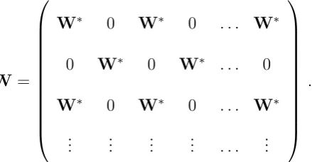
λ0i, λ1i and λ2i are generated from U(−0.6,0.6). The spatial weight matrix W used is a block diagonal matrix formed by a √p× √p row-normalized matrix W∗. We construct W∗ such that the first four sub-diagonal elements are all 1 and the rest elements are all 0 before normalizing. This kind of W corresponds to the pooling of √p separate districts with similar neighboring structures in each district, see Lee and Yu (2013), that is

W=

               

W∗ 0 0 . . . 0 0 W∗ 0 . . . 0 0 0 W∗ . . . 0

..

. ...

0 0 0 . . . W∗

               

.

The error εi,t are independently generated from N(0, σ2i), where we generate each σi from U(0.5,1.5).

For all scenarios, we generate data from (1.2.1) with different settings for n and p. We apply the proposed estimation method (1.2.3) and (1.2.5) (with di = min (p, n10/21)) and report the mean absolute errors:

MAE(i) = 1 3

2

∑

j=0

|bλji−λji|, MAE = 1 p

p

∑

i=1

We replicate each setting 500 times.

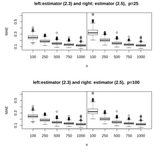
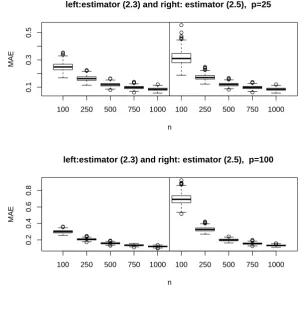
Figure 1.2 depicts two boxplots of MAE with p equals to, respectively, 25 and 100. As the sample size n increases from 100, 250, 500, 750 to 1000, MAE decreases for both methods.

100 250 500 750 1000 100 250 500 750 1000

0.1

0.3

0.5

left:estimator (2.3) and right: estimator (2.5), p=25

n

MAE

100 250 500 750 1000 100 250 500 750 1000

0.1

0.3

0.5

left:estimator (2.3) and right: estimator (2.5), p=100

n

MAE

Figure 1.2: Boxplots of MAE for estimator (1.2.3) (left panels) and estimator (1.2.5) (right panels) with p = 25 (top panels) and 100 (bottom panels), n = 100, 250, 500, 750, 1000 for scenario 1.

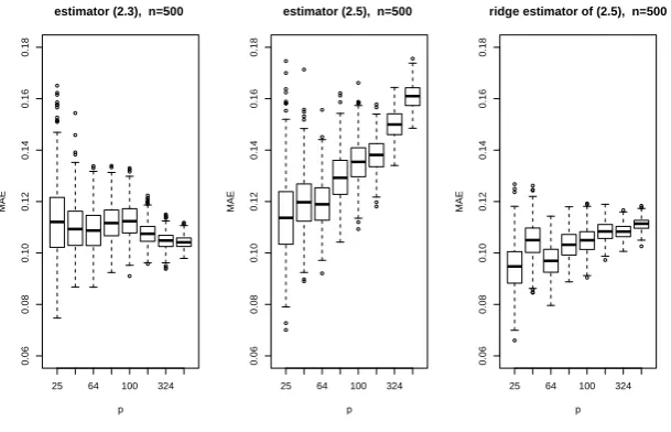
Figure 1.3 depicts the boxplots of the MAE for the original estimator (1.2.3), the root n consistent estimator (1.2.5), and the estimator (1.2.5) with the ridge penalty, where we choose the ridge tuning parameter to be C × _np in order to avoid the nearly singularity problem of ZbT

set at 25,49,64,81,100,169,324 and 529 respectively. The MAE for (1.2.3) remains about the same level aspincreases; see the panel on the left in Figure 1.3. This is in line with the asymptotic result of Theorem 4 when, for example,s1(p)≍C,s0(p)≍pand s2(p)≍p. In

contrast, the MAE for estimator (1.2.5) increases sharply when p increases; see the panel in the middle. This is due to the fact that ZbT

iZbi is nearly singular for large p. Adding a ridge in the estimator certainly mitigates the deterioration when pincreases; see the panel on the right in Figure 1.3.

25 64 100 324

0.06

0.08

0.10

0.12

0.14

0.16

0.18

estimator (2.3), n=500

p

MAE

25 64 100 324

0.06

0.08

0.10

0.12

0.14

0.16

0.18

estimator (2.5), n=500

p

MAE

25 64 100 324

0.06

0.08

0.10

0.12

0.14

0.16

0.18

ridge estimator of (2.5), n=500

p

MAE

Figure 1.3: Boxplots of MAE of the original estimator (1.2.3) (the left panel), the root n consistent estimator (1.2.5) (the middle panel), and the estimator (1.2.5) after adding ridge penalty (the right panel) with n= 500 andp= 25,49,64,81,100,169,324,529 for scenario 1.

1.4.2

Scenario 2

W∗ is chosen such that the first two sub-diagonal elements are all 1 and the rest elements are all 0 before normalizing. Then we treat W as a √p× √p block matrix and put W∗ into the main diagonal, 2nd, 4th, 6th and etc. sub-diagonal block positions. This kind of W corresponds to the pooling of √p districts (each district has √p locations) which the evenly numbered districts are connected and the oddly numbered districts are connected but evenly numbered districts and oddly number districts are separated. Each district has similar neighboring structures. Asp increases, the number of the locations influencing one specific location increases in the order of √p, that is

W =

           

W∗ 0 W∗ 0 . . . W∗ 0 W∗ 0 W∗ . . . 0 W∗ 0 W∗ 0 . . . W∗

..

. ... ... ... . . . ...

           

.

The error εi,t are independently generated from N(0, σ2i), where we generate each σi from U(0.5,1.5).

Figure 1.4 depicts two boxplots of MAE with p equals to, respectively, 25 and 100. As the sample size n increases from 100, 250, 500, 750 to 1000, MAE decreases for both methods.

Figure 1.5 depicts three boxplots as Figure 1.3. The MAE for (1.2.3) increases steadily as p increases, which matches the result of Theorem 4 when, for instance, s1(p) ≍ √p,

s0(p)≍pands2(p)≍p. The MAE for (1.2.5) after adding ridge penalty is slowly increasing

as well. This might be caused by the fact that, similar to A2(c), quantities in condition A4(a) is also influenced by psince the number of nonzero elements in wi is in the order of

√

100 250 500 750 1000 100 250 500 750 1000

0.1

0.3

0.5

left:estimator (2.3) and right: estimator (2.5), p=25

n

MAE

100 250 500 750 1000 100 250 500 750 1000

0.2

0.4

0.6

0.8

left:estimator (2.3) and right: estimator (2.5), p=100

n

MAE

Figure 1.4: Boxplots of MAE for estimator (1.2.3) (left panels) and estimator (1.2.5) (right panels) with p = 25 (top panels) and 100 (bottom panels), n = 100, 250, 500, 750, 1000 for scenario 2.

1.5

Real data analysis

1.5.1

European Consumer Price Indices

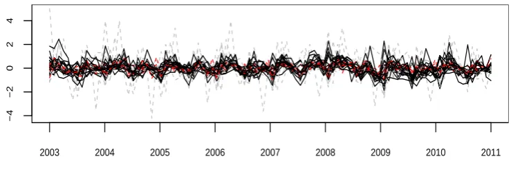
We analyze the monthly change rates of the consumer price index (CPI) for the EU member states, over the years 2003-2010. We use the national harmonized index of consumer prices calculated by Eurostat, the statistical office of the European Union. For this data set, n= 96 and p= 31.

25 64 100 324

0.1

0.2

0.3

0.4

0.5

0.6

estimator (2.3), n=500

p

MAE

25 64 100 324

0.1

0.2

0.3

0.4

0.5

0.6

estimator (2.5), n=500

p

MAE

25 64 100 324

0.1

0.2

0.3

0.4

0.5

0.6

ridge estimator of (2.5), n=500

p

MAE

Figure 1.5: Boxplots of MAE of the original estimator (1.2.3) (the left panel), the root n consistent estimator (1.2.5) (the middle panel), and the estimator (1.2.5) after adding ridge penalty (the right panel) with n= 500 andp= 25,49,64,81,100,169,324,529 for scenario 2.

2003 2004 2005 2006 2007 2008 2009 2010 2011

−4

−2

0

2

4

Figure 1.6: Time series plots of the monthly change rates of CPI for the 31 EU member states. Each series is subtracted by its mean value.

states. To line up the curves together, each series is centered at its mean value in Figure 1.6. There exist clearly synchronizes on the fluctuations across different states, indicating the spatial (i.e. cross-state) correlations among different states. Also noticeable is the varying degrees of the fluctuation over the different states.

spatial-temporal model (1.2.1) to this data set with the parameters estimated by (1.2.3). We take a normalized sample correlation matrix of yt as the spatial weight matrixW = (wij), i.e. we let wij be the absolute value of the sample correlation between the i-th and j-th states for i̸=j, and wii= 0, and then replace wij bywij/

∑

kwkj.

Figure 1.7 presents the scatter plots of yi,t against, respectively, the 3 regressors in model (1.2.1), i.e. wT_i yt, yi,t−1, wTi yt−1, for four selected states Belgium, Greece, France

and Iceland. We superimpose the straight line y = bλjix in each of those 3 scatter plots with, respectively, j = 0,1,2. It is clear that the estimated slopes are very different for those 4 states. Figure 1.8 plots the true monthly change rates of the CPI for those 4 states together with the fitted values

b

yi,t =bλ0iwTi yt+bλ1iyi,t−1 +bλ2iwiTyt−1. (1.5.12)

−2 −1 0 1 2 −3 −2 −1 0 1 2 3 Belgium

wiyt

yit

−2 −1 0 1 2

−3 −2 −1 0 1 2 3 Greece

wiyt

yit

−2 −1 0 1 2

−3 −2 −1 0 1 2 3 France

wiyt

yit

−2 −1 0 1 2

−3 −2 −1 0 1 2 3 Iceland

wiyt

yit

−2 −1 0 1 2

−3 −2 −1 0 1 2 3 Belgium

yi(t−1)

yit

−2 −1 0 1 2

−3 −2 −1 0 1 2 3 Greece

yi(t−1)

yit

−2 −1 0 1 2

−3 −2 −1 0 1 2 3 France

yi(t−1)

yit

−2 −1 0 1 2

−3 −2 −1 0 1 2 3 Iceland

yi(t−1)

yit

−2 −1 0 1 2

−3 −2 −1 0 1 2 3 Belgium

wiyt−1

yit

−2 −1 0 1 2

−3 −2 −1 0 1 2 3 Greece

wiyt−1

yit

−2 −1 0 1 2

−3 −2 −1 0 1 2 3 France

wiyt−1

yit

−2 −1 0 1 2

−3 −2 −1 0 1 2 3 Iceland

wiyt−1

yit

Figure 1.7: The scatter plots of yi,t againstwTi yt (panels on the top), yi,t−1 (panels in the

middle), and wT

i yt−1 (panels on the bottom) for four selected countries Belgium, Greece,

France and Iceland. The straight lines y=bλjix are superimposed in the panels on the top with j = 0, those in the middle with j = 1, and those on the bottom with j = 2.

Belgium

−3

−1

1

3

Greece

−3

−1

1

3

Fr

ance

−3

−1

1

3

Iceland

−3

0

2

2003 2004 2005 2006 2007 2008 2009 2010 2011

Figure 1.8: The monthly change rates of CPI (thin lines) of Belgium, Greece, France and Iceland, and their estimated values (thick lines) by model (1.2.1).

Gener. YW Const. QML

−0.4

−0.3

−0.2

−0.1

0.0

0.1

0.2

0.3

Out−of−sample forecasts (leaving out 6) Average Error

Gener. YW Const. QML

0.0

0.2

0.4

0.6

0.8

1.0

1.2

Out−of−sample forecasts (leaving out 6) Average Square Error

Figure 1.9: Prediction errors generated in the out-of-sample forecasting, leaving out 6 observa-tions from the sample, using our model with the Generalized Yule-Walker estimator and using

the constant SDPD model of Yu et al. (2008) with the Quasi-Maximum Likelihood estimator.

To further vindicate the necessity to use different coefficients for different states, we consider a statistical test for hypothesis

for model (1.2.1). Then the residuals resulting from the fitted model under H0 will be

greater than the residuals without H0. However if H0 is true, the difference between the

two sets of residuals should not be significant. We apply a bootstrap method to test this significance. Let eλ0,eλ1,λe2 be the estimates under hypothesisH0. Define the test statistic

U = 1 n

n

∑

t=1

∥yt−yet∥1, yet=eλ0Wyt+eλ1yt−1+eλ2Wyt−1.

We reject H0 for large values of U. To assess how large is large, we generate a bootstrap

data from

y∗_t =eλ0Wyt+eλ1yt−1 +eλ2Wyt−1 +ε∗t,

where {ε∗_t} are drawn independently from the residuals

bεt=yt−byt, t= 1,· · · , n,

andbytconsists of the components defined in (1.5.12). Now the bootstrap statistic is defined as

U∗ = 1 n

n

∑

t=1

∥y∗_t −(λ∗₀Wyt+λ∗₁yt₋1+λ∗2Wyt−1)∥1,

where (λ∗₀, λ∗₁, λ∗₂) is the estimated coefficients for the regression model

y∗_t =λ0Wyt+λ1yt−1+λ2Wyt−1+εt, t = 1,· · · , n. The P-value for testing hypothesis H0 is defined as

P(U∗ > U|y1,· · ·,yn),

which is approximated by the relative frequency of the event (U∗ > U) in a repeated bootstrap sampling with a large number of replications. By repeating bootstrap sampling 1000 times, the estimatedP-value is 0, exhibiting strong evidence against the null hypoth-esis H0. Therefore the model with the equal slope parameters across different locations is

1.5.2

Modeling mortality rates

Now we analyze the annual Italian male and female mortality rates for different ages (be-tween 0 and 104) in the period of 1950 – 2009 based on the proposed model (1.2.1). The data

were downloaded from the Human Mortality Database (see the website http://www.mortality.org/). Let mi,t be the log mortality rate of female or male at age i and in Year t. Those data

are plotted in Figure 1.10. Two panels on the left plot are the female and male mortal-ity against different age in each year. More precisely the curves {mi,t, i = 1,· · · ,21} for t < 1970 are plotted in red, those for t > 1990 are in blue, those with 1970 ≤ t ≤ 1989 are in grey. Those curves show clearly that the mortality rate decreases over the years for almost all age groups (except a few outliers at the top end). Two panels in the middle of Figure 1.10 plot the log mortality for each age group against time with the following color code: black for ages not great than 10, grey for ages between 11 and 100, and green for ages greater than 100. They indicate that the mortality for all age groups decreases over time, the most significant decreases occur at the young age groups. Furthermore, the fluctuation of the mortality rates for the top age groups reduces significantly over the years, while the mean mortality rates for those groups remain about the same. This can be seen more clearly in the two panels on the right which plot differenced log mortality rates

{yi,t, t= 1951,· · ·,2009}, using the same colour code, where yi,t =mi,t−mi,t−1.

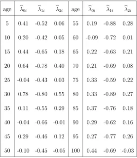
We fit the differenced log mortality data with model (1.2.1) with the parameters esti-mated by (1.2.5) and di = 20. Note that now p = 104 and n = 59. Let the off-diagonal elements of the spatial weight matrixW be

wij = 1

Female log death rates

age

before 1970 after 1990

−10

−8

−6

−4

−2

0

0 9 19 31 43 55 67 79 91

Female log death rates

time

<10 years >100 years

−10

−8

−6

−4

−2

0

1950 1961 1972 1983 1994 2005

lag differences

time

−0.5

0.0

0.5

1951 1962 1973 1984 1995 2006

Male log death rates

age

−10

−8

−6

−4

−2

0

0 9 19 31 43 55 67 79 91

Male log death rates

time

−10

−8

−6

−4

−2

0

1950 1961 1972 1983 1994 2005

lag differences

time

−4

−2

0

2

4

1951 1962 1973 1984 1995 2006

Figure 1.10: Log mortality rates of Italian female (3 top panels) and male (3 bottom panels) are plotted against age from each year in 1950-2009 (2 left panels), against year for each age group

between 0 and 104 (2 middle panels). Differenced log mortality rates are plotted against year for

each age in 2 right panels.

We then replacewij bywij/∑_iwij. Moreover, we can also fix a thresholdτ and set to zero all the elements of matrix W such that |x−w| > τ (for simplicity, we fix τ = 5 in this application, but the results are substantially invariant for different values of τ).

age bλ0i bλ1i bλ2i age bλ0i bλ1i bλ2i 5 0.41 -0.52 0.06 55 0.19 -0.88 0.28 10 0.20 -0.42 0.05 60 -0.09 -0.72 0.01 15 0.44 -0.65 0.18 65 0.22 -0.63 0.21 20 0.64 -0.78 0.40 70 0.21 -0.69 0.08 25 -0.04 -0.43 0.03 75 0.33 -0.59 0.22 30 0.78 -0.80 0.55 80 0.33 -0.89 0.27 35 0.11 -0.55 0.29 85 0.37 -0.76 0.18 40 -0.04 -0.66 -0.01 90 0.29 -0.62 0.16 45 0.29 -0.46 0.12 95 0.27 -0.77 0.26 50 -0.10 -0.45 -0.05 100 0.44 -0.69 -0.03

Table 1.1: Estimated coefficients for a selection of cohorts of different ages. The left column

is the estimated pure spatial coefficients bλ0i; The middle column is the estimated pure dynamic

coefficientλb1i; The right column is the estimated spatial-dynamic coefficients bλ2i.

1.6

Final remark

Age 60

−0.3

0.1

Age 80

−0.3

0.1

Age 100

−0.3

0.1

1961 1965 1969 1973 1977 1981 1985 1989 1993 1997 2001 2005 2009

Figure 1.11: Observed time series (thin line) and fitted time series (bold line), for female mortality

rate for agesi= 60,80,100.

1.7

Appendix: Proofs

We present the proofs for Theorems 2, Corollary 1 and Theorem 4 in this appendix. The proofs for Theorem 1 and 3 are similar and simpler than that of Theorem 2, and they are therefore omitted. We also present a lemma (i.e. Lemma 1) at the end of this appendix, which shows that condition A2 is implied by conditions A1 and B1 – B3; see Remark 1. We use C to denote a generic positive constant, which may be different at different places.

(1) √ nU− 1 2 i         1 n ∑n

t=1y

T

t−1(wTi yt)_n1

∑n

t=1εi,tyt−1 1

n

∑n

t=1y

T

t−1yi,t−11_n

∑n

t=1εi,tyt−1 1

n

∑n

t=1yTt−1(wTi yt−1)_n1

∑n

t=1εi,tyt−1

        d −

→N(0,I3).

(2) Vi(XbTi Xbi)−1 P

−→I3.

To prove (1), it suffices to show that for any nonzero vectora= (a1, a2, a3)T, the linear

combination aT         1 n ∑n

t=1y

T

t−1(wiTyt)_n1

∑n

t=1εi,tyt−1 1

n

∑n

t=1y

T

t−1yi,t−1_n1

∑n

t=1εi,tyt−1 1

n

∑n

t=1ytT−1(wiTyt−1)_n1

∑n

t=1εi,tyt−1

       

is asymptotic normal.

Let us take out the dominant term in 1_n∑n_t=1yT

t−1(wTi yt)_n1

∑n

t=1εi,tyt−1 first.

1 n

n

∑

t=1

yT_t−1(wT_i yt) 1 n

n

∑

t=1

εi,tyt−1

= [ 1 n n ∑ t=1

yTt−1(wTi yt)−E[ytT−1(wiTyt)]

] 1 n n ∑ t=1

εi,tyt₋1+ E[ytT−1(w

T i yt)] 1 n n ∑ t=1

εi,tyt₋1

= [ 1 n n ∑ t=1

yT_t−1(wT_i yt)−wTi Σ1

] 1 n n ∑ t=1

εi,tyt−1+

1 n

n

∑

t=1

wT_i Σ1yt−1εi,t

=E1+E2.

For termE1 and k= 1,2,· · · , p, by Proposition 2.5 of Fan and Yao (2003), we have E [ 1 n n ∑ t=1

(eT_kyt−1wTi yt−eTkΣ T

1wi)

]2 = 1 n2 n ∑ t=1

Var(eT_kyt−1wTi yt) + 1 n2

∑

t̸=s

Cov(eT_kyt−1wTi yt,eTkys−1wTi ys)

≤C

n + 1 n2

∑

t̸=s

8α(|t−s|)4+γγ

[

E|eT_kyt₋1wiTyt|

2+γ₂]

2 4+γ[

E|eT_kys₋1wTi ys|

2+γ₂]

2 4+γ ≤C n + C n2 ∑

t̸=s

α(|t−s|)4+γγ ≤ C

n + C n n ∑ j=1

α(j)4+γγ =O(1

n),

(1.7.14)

where C is independent of p. Then it holds that 1

n n

∑

t=1

(e_kTyt−1wiTyt−eTkΣ T

1wi) =Op( 1 √ n). Therefore 1 n n ∑ t=1

yt−1wiTyt−ΣT1wi

2 = v u u

t∑p

k=1 [ 1 n n ∑ t=1 (eT

kyt−1w T

i yt−eT_kΣT1wi)

]2

=Op(

√ p n). Similarly, 1 n n ∑ t=1

εi,tyt−1

2

=Op(

√

p n). Since E1 ≤ _n1

∑n

t=1yt−1w

T

i yt−ΣT1wi_2n1

∑n

t=1εi,tyt−12, it holds that E1 = Op(

p n). Similar to (1.7.14), we have Var(√nE2) = O(1). Given √p_n = o(1), it holds that

√

nE1 =

op(1). Hence ifp=o(

√

n),

√

n× 1 n

n

∑

t=1

yT_t−1(wT_i yt) 1 n

n

∑

t=1

εi,tyt−1 =

1 √ n n ∑ t=1

wT_i Σ1yt−1εi,t+op(1).

Similarly, given p=o(√n), we have

√

n× 1 n

n

∑

t=1

yT_t−1yi,t−1

1 n

n

∑

t=1

εi,tyt−1 =

1 √ n n ∑ t=1

eT_i Σ0yt−1εi,t+op(1),

√

n× 1 n

n

∑

t=1

yT_t−1(wT_i yt₋1)

1 n

n

∑

t=1

εi,tyt₋1 =

1 √ n n ∑ t=1

Now it suffices to prove

Sn,p ≡a1

1 √ n n ∑ t=1

w_iTΣ1yt−1εi,t+a2

1 √ n n ∑ t=1

eT_i Σ0yt−1εi,t+a3

1 √ n n ∑ t=1

w_iTΣ0yt−1εi,t

is asymptotic normal. Note that it holds that

E|wT_i Σ1yt−1εi,t|2+

γ

2 ≤[E|wT

i Σ1yt−1)4+γ|

1

2[E|ε_i,t|4+γ] 1 2 <∞.

Now we calculate the variance of Sn,p. It holds that

Var ( 1 √ n n ∑ t=1

w_iTΣ1yt−1εi,t

)

=wT_i Σ1Σy,εi(0)Σ

T

1wi+ n−1

∑

j=1

(

1− j n

)

wT_i Σ1

[

Σy,εi(j) +Σ

T

y,εi(j)

]

ΣT₁wi,

(1.7.15)

and it follows from ∑n_j=1α(j)4+γγ _<∞ _that

sup p

∞ ∑

j=1

|wT_i Σ1

[

Σy,εi(j) +Σ

T

y,εi(j)

]

ΣT₁wi|

≤Csup p

∞ ∑

j=1

α(j)4+γγ {_E|_wT

i Σ1yt−1|4+γ

} 2

4+γ{_E|_εi,t|4+γ}

2

4+γ _<∞_.

Similarly, Cov ( 1 √ n n ∑ t=1

w_iTΣ1yt−1εi,t, 1 √ n n ∑ t=1

eT_i Σ0yt−1εi,t

)

=wT_i Σ1Σy,εi(0)Σ

T

0ei+ n−1

∑

j=1

(

1− j n

)

w_iTΣ1

[

Σy,εi(j) +Σ

T

y,εi(j)

]

Σ0ei,

and sup_p∑∞_j=1|wT

i Σ1Σy,εi(j)Σ0ei|< ∞. Calculating all the variance and covariance and

summing up them, it follows from dominate convergence theorem that

Var

(

Sn,p

√

aT_U ia

)

→1.