2019 International Conference on Computational Modeling, Simulation and Optimization (CMSO 2019) ISBN: 978-1-60595-659-6
Bee Spices Transition with Rapid Global Optimization Algorithm
Xu-ming HAN
1, Lin-lin WANG
1, Li ZHENG
1,
Yuan-yuan DANG
1and Li-min WANG
2,*1School of Computer Science and Engineering, Changchun University of Technology, 2055 Yanan Street, Changchun 130012, China
2School of Management Science and Information Engineering, Jilin University Finance and Economics Changchun, 3699 Jingyue Street, Changchun 130117, China
*Corresponding author
Keywords: Bee spices transition, Function optimization, Meta heuristic, Artificial bee colony,
Dynamic economic dispatch.
Abstract. Swarm intelligence algorithm is a general term for a class of intelligent groups with self-organized behavior. A novel Artificial Bee Colony algorithm is introduced in this paper, named Bee Spices Transition with Rapid Global Optimization Algorithm (BSTRGOA). The contribution of BSTRGOA algorithm consists of two parts. First, the evolution strategy of bee species balances the global exploration ability and the local search ability. Second, the fast search mechanism of global optimization is proposed. It reinforces global learning of the colony. The BSTRGOA algorithm is experimented with the CEC 2017 benchmark functions. It shows the BSTRGOA algorithm can effectively improve the convergence speed and optimization accuracy. And the BSTRGOA algorithm has a good performance in solving the problem of multi-dimensional function optimization. In addition, BSTRGOA algorithm is also applicable to dynamic economic scheduling analysis, and the conclusion also shows it can significantly improve the time efficiency.
Introduction
The artificial bee colony algorithm was proposed by D. Karaboga in 2005. At present, it is applied to solve practical optimization problems such as neural network [1], clustering analysis [2] and vehicle routing problem [3]. In recent years, ABC algorithm has attracted extensive attention of scholars. D. Karaboga et al. [4] compared the performance of ABC algorithm with particle swarm optimization (PSO), differential evolution algorithm (DE) and evolutionary algorithm (EA) under different control parameters. The simulation results showed that the ABC algorithm was better than the above algorithms. In order to enlarge the neighborhood and expand the search space [5-7], D.L. Zhang et al. [8] proposed the improved ABC algorithm based on multi-exchange neighborhood based on the characteristics of multi-exchange neighborhood structure.
The Artificial Bee Colony Algorithm
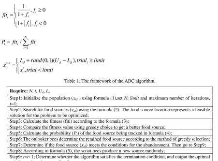
The ABC algorithm consists the employed bees, the onlooker bees and the scout bees. Among them, the employed bees and the onlooker bees account for one-half of the all bees [9]. Table 1 shows the framework of the ABC algorithm. N represents the population of nectar sources, d represents the dimension. Trial represents the number of iterations. Limit represents the search threshold.
(0,1)( )
id d d d
x L rand U L (1)
id id id jd
1
, 0 1
1 , 0
i i i
i i
f f fit
f f
(3)
1 N
i i i
i
P fit fit
(4)1 (0,1)( ),
,
d d d i
t
i t
i
L rand U L trial limit x
x trial limit
[image:2.595.70.522.69.402.2] (5)
Table 1. The framework of the ABC algorithm.
Require: N, t, Ud, Ld
Step1: Initialize the population (xid) using formula (1),set N; limit and maximum number of iterations,
t=1;
Step2: Search for food sources (vid) using the formula (2). The food source location represents a feasible
solution for the problem to be optimized;
Step3: Calculate the fitness (fiti) according to the formula (3);
Step4: Compare the fitness value using greedy choice to get a better food source; Step5: Calculate the probability (Pi) of the food source being tracked in formula (4);
Step6: The onlooker bees determine the retained food source according to the method of greedy selection; Step7: Determine if the food source (xid) meets the conditions for the abandonment. Then go to Step9;
Step8: According to formula (5), the scout bees produce a new source randomly;
Step9: t=t+1; Determine whether the algorithm satisfies the termination condition, and output the optimal solution, otherwise go to Step2.
Bee Spices Transition with Rapid Global Optimization Algorithm
When solving actual optimization problems, the solution space is complex and multi-modal. According to formula (5), we found that the algorithm lacks the ability to mutate when the threshold limit is reached which easily leads to the low precision of local search and leads the bee to fall into local extremum. So the evolution strategy of bee species and the fast searching mechanism of global optimization are proposed.
Evolution Strategy of Bee Species. In BSTRGOA, the evolution strategy of bee species is proposed. In the early stage of the iteration, the employed bees search for the global extraction of food sources, which account for a high proportion. But in the later stage of iteration, the proportion of the onlooker bees increase and the local exploration ability is enhanced, which provide a guarantee to obtain a better food source. is a random number in [0,1] in formula(6).
2 ( ) 1 * t p t
T
(6) The employed bees’ number is expressed as the product of the total number of bees and the p(t) function. In early stage of the iteration, the global search ability is enhanced. In the latter stage of the iteration, the p(t) function descended faster, the search of the employed bees is decreased. The number of the onlooker bees increases. It enhances the local search capability.
1 ( ) (0,1)( ), ,
d d i
t
i t
i
M t rand U L trial limit x
x trial limit
(7)
( ) sin ( / 2)*( / ) 1.5 * tfitnessbest
M t t T x
(8) In formula (7), the function M(t) is introduced. Among them, xtfitnessbestrepresents the food source
with the best fitness searched in the previous iteration. The value range of
( ) sin ( / 2)*( / ) 1.5 * tfitnessbest
M t t T x function is (0,1). In the early stage of the iteration, the
sin ( / 2)*( / ) 1.5 t T function has a lower slope, and the weight increases with the number of
iterations. In the late iteration period, the function has a large slope, and the weight of the optimal solution of the previous generation increases accordingly. Therefore, the dynamic proportion of the previous generation’s optimal solution has been changed.
[image:3.595.146.451.616.729.2]The Framework of Bee Spices Transition with Rapid Global Optimization Algorithm. The specific flow of the BSTRGOA algorithm is as follows in Table 2.
Table 2. The framework of the BSTRGOA algorithm.
Require: N, t, Ud, Ld
Step1: Initialize the population (xid ) using formula (1) and formula (6),set parameters N; limit and
maximum number of iterations, t=1;
Step2: Search for food sources (vid) using the formula (2);
Step3: Calculate the fitness (fiti) according to the formula (3);
Step4: Compare the fitness value using greedy choice to get a better food source; Step5: Calculate the the food source’s probability (Pi) in formula (4);
Step6: The onlooker bees determine the retained food source according to the method of greedy selection; Step7: Determine if xid meets the conditions for the abandonment. Then go to Step9;
Step8: According to formula (7) and formula (8), the scout bees randomly produce a new source randomly;
Step9: t=t+1; Determine whether the algorithm satisfies the termination condition, and output the optimal solution, otherwise go to Step2.
Simulation Experiment and Analysis. 6 CEC functions are used in solving single-objective real-value optimization problem. Table 3 briefly described the 6 functions with different characteristics. Fig.1 shows the three-dimensional topographic map of the functions. The benchmark function is a minimization problem. For a detailed introduction of the CEC2017 single objective real value test set, please refer to [10]. Simulation experiment environment is processor for the Inter(R) Core (TM) i5-4590S3.00GHZ, 8GB memory PC, operating system Windows7 Ultimate 64-bit operating system, programming software for the MATLAB R2014a. BSTRGOA algorithm is compared with the ABC algorithm, EABC algorithm, HABC algorithm and GABC algorithm.
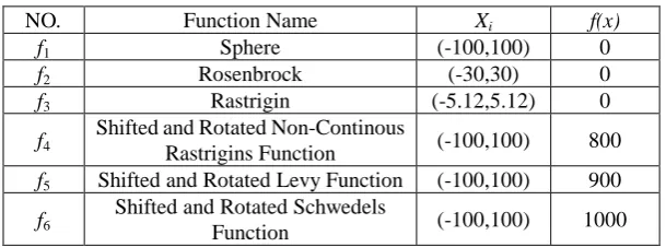
Table 3. Benchmark Functions.
NO. Function Name Xi f(x)
f1 Sphere (-100,100) 0
f2 Rosenbrock (-30,30) 0
f3 Rastrigin (-5.12,5.12) 0
f4
Shifted and Rotated Non-Continous
Rastrigins Function (-100,100) 800 f5 Shifted and Rotated Levy Function (-100,100) 900 f6
Shifted and Rotated Schwedels
Figure 1. 6 benchmark functions(first row: f1—f3,second row: f4—f6).
Experimental Design
[image:4.595.83.514.369.569.2]The experiment sets the parameters of the Benchmark function, as shown in Table 3. There are five kinds of comparison methods, (1) ABC (2) EABC[11] (3) GABC[12] (4) HABC[13] (5) BSTRGOA. The experimental parameters are set as follows: Tmax=1000, sizepop=30, Dim=50, and runtime=50.
Table 4. Results of 5 algorithms (sizepop=30).
Function Algorithm Min Max Mean Std
ƒ1
ABC 1.4689E-03 6.2843E+04 4.7338E+03 1.3941E+08 EABC 7.2383E-10 2.0794E+04 9.3882E+02 8.9817E+06 GABC 5.5107E-16 9.5128E+03 9.3233E+01 4.6211E+05 HABC 2.2941E-13 2.3188E+03 9.4147E+00 1.4798E+04 BSTRGOA 5.2742E-16 1.4321E+04 2.2227E-05 1.7969E-06
ƒ2
ABC 1.5005E+02 2.8260E+08 1.5429E+07 2.4449E+15 EABC 2.8765E+00 7.3904E+06 1.4457E+05 5.8411E+11 GABC 3.8199E+00 1.3613E+07 1.3952E+05 1.1164E+12 HABC 3.1939E-03 1.0491E+06 4.4908E+03 4.2037E+09 BSTRGOA 2.0090E-16 5.0259E+03 4.6584E-04 1.3796E-05
ƒ3
ABC 8.7613E+00 4.7029E+02 7.7356E+01 9.1923E+03 EABC 9.9498E-01 1.9933E+02 1.9013E+01 1.1583E+03 GABC 2.1927E-10 1.5390E+02 5.1921E+00 2.0478E+02 HABC 1.8758E-12 3.6220E+01 1.0512E+00 1.1335E+01 BSTRGOA 2.0443E-16 4.5853E+03 4.2720E-01 1.1774E-05
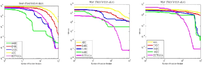
Experimental Precision Analysis. The results in Table 4 show that the BSTRGOA algorithm is better in functions f2, the optimization precision of BSTRGOA algorithm is significantly improved,
reaching 10-16. It improves the accuracy of the algorithm.
[image:4.595.134.462.623.735.2]convergence speed. On the other hand, it proves that BSTRGOA has strong global search ability and local development ability in solving multidimensional function optimization problems.
[image:5.595.70.533.163.351.2]Comparison with Other Meta-heuristic Algorithms. Compared with other four algorithms(CS, PSO, FWA [14], ABC) in Table 5, the BSTRGOA algorithm is improved by an average of 4 orders of magnitude. In the experiment, Dim=50, Tmax=1000, and runtime=50.
Table 5. Results of 5 Meta-heuristic Algorithms (sizepop = 30).
Fun
CS PSO FWA ABC BSTRGOA
Media
n Std
Media
n Std
Media
n Std
Media
n Std
Media
n Std
ƒ1 1.7970 E-01 9.0300 E-02 2.0000 E+01 1.5995 E-03 2.3823 E+01 1.0836 E-04 1.1203 E+03 5.4910 E-01 8.5747 E-05 1.8013 E-06 ƒ2 5.5312 E+02 2.8920 E+02 4.2560 E+03 3.5488 E-01 4.6720 E+03 3.3613 E+01 6.5481 E+07 1.7948 E+02 4.9518 E-04 3.6738 E-05 ƒ3 1.5298 E+02 2.0219 E+01 3.9617 E+02 5.2891 E-02 4.0314 E+02 2.9278 E+00 4.5975 E+01 5.5668 E+00 1.0102 E-01 3.3944 E-05 ƒ4 1.2593 E+03 1.5497 E+02 1.6775 E+03 1.5924 E-02 3.1482 E+03 6.3248 E+03 1.1523 E+03 3.3321 E+01 1.1594 E+02 1.9825 E+01 ƒ5 3.2305 E+04 1.3536 E+04 5.4468 E+04 2.2567 E-01 6.5219 E+03 2.8825 E+03 2.2468 E+04 3.1420 E+03 1.8949 E+02 4.6385 E+03 ƒ6 1.0196 E+04 1.6563 E+03 2.0338 E+04 1.0919 E-01 3.1129 E+03 5.4923 E+03 8.0070 E+03 3.2803 E+02 7.8952 E+02 2.7625 E+02
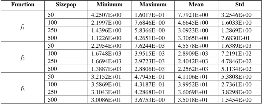
The Effect of Different Population Sizes. Table 6 shows the search accuracy of the BSTRGOA algorithm for a population size of 50, 100, 250, and 500. The time complexity of the BSTRGOA algorithm is O(tN2). As the population size increases, the BSTRGOA algorithm still shows good optimization performance.
Table 6. Results of different population size.
Function Sizepop Minimum Maximum Mean Std
f1
50 4.2507E+00 1.6017E+01 7.7921E+00 3.2546E+00 100 2.1997E+00 7.6846E+00 4.6645E+00 1.6033E+00 250 1.4396E+00 5.8366E+00 3.0923E+00 1.2869E+00 500 1.1226E+00 4.2651E+00 3.3065E+00 7.6830E-01
f2
50 2.2954E+00 7.6244E+03 4.5578E+00 1.6389E+03 100 1.6748E+03 3.9515E+03 2.8909E+03 7.2191E+02 250 1.6694E+03 2.9723E+03 2.4042E+03 4.7846E+02 500 1.3887E+03 2.8806E+03 2.2562E+03 5.1134E+02
f3
50 3.2152E+01 4.7945E+01 4.1106E+01 5.3808E+00 100 3.5869E+01 4.3187E+01 3.9952E+01 2.7361E+00 250 3.1043E+01 4.2868E+01 3.6069E+01 3.8298E+00 500 3.0086E+01 3.6753E+00 3.5018E+01 1.5454E+00
Applications
The characteristics of power system dispatching changing with time are more and more obvious [15]. The ABC algorithm is applied into the power system economic dispatching problem, which has a strong practical significance and economic value [16].
Research Background. The Dynamic Economic Dispatch (DED) problem follows the characteristics of the hourly dispatch problem [17]. 5 generating units’ power system data are used to evaluate the optimization ability. There are 2 kinds of comparison methods, (1) ABC (2) BSTRGOA. The objective function corresponding to the production cost is represented as:
( )
G
N T
c ih ih
F F P
[image:5.595.83.515.435.608.2]2 min
( ) sin( ( ))
it it i it i it i i it it it
F P a P b P c e f P P (10)
i=1, 2, 3,…NG. Pit is the real power output (in MW) , NG is the number of online generating units, T
is the dispatching time. The power balance constraints are:
1
G
N
it Dt Lt
i
P P P
(11) B-coefficients is calculated to get PLt, given by1 1
G G
N N
Lt it ij jt
i j
P P B P
(12)The generator constraint is as follows:
min max
i it i
P P P (13)
Pimin =lower bound, Pimax = upper bound, for power outputs of the ith generating unit in MW. The
rates of each unit’s rise and fall satisfy the following constraints: If power generation increased:
1 t
it i i
P P UR (14) If power generation decreased:
1 t
i it i
P P DR (15)
Pit-1 represents the previous hour’s power generation, URi represents the upper ramp limit, and DRi
represents the lower ramp rate limits respectively. Experiments use the following fitness function model to simulate:
2 2
1 lim
1 1 1 1 1 1
( )
n N n N n N
k i it it Dt r it r
t i t i t i
f F P P P P P
(16) λ1 and λr are penalty parameters, n represents the hours’ number, N represents the units’ number.The Prlim was defined by
( 1) ( 1)
lim ( 1) ( 1) ,
,
,
i t i it i t i
r i t i it i t i
it
P DR P P DR
P P DR P P DR
P otherwise
(17)
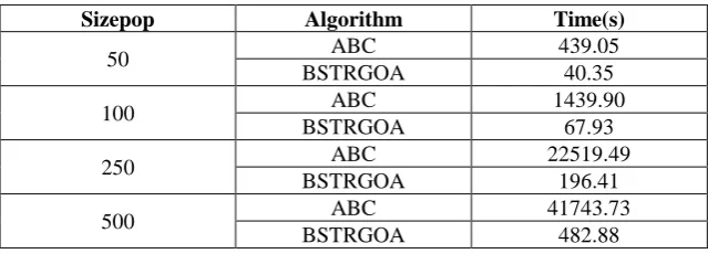
Time Comparison of Algorithm in Application. When the population size is 50, 100, 250 and 500, each algorithm runs 50 times independently under the condition that the Dim=50 and Tmax =1000.
[image:6.595.138.458.658.773.2]The data in Table 7 show that the BSTRGOA algorithm improves the search efficiency and saves search time.
Table 7. Time results of two algorithms.
Sizepop Algorithm Time(s)
50 ABC 439.05
BSTRGOA 40.35
100 ABC 1439.90
BSTRGOA 67.93
250 ABC 22519.49
BSTRGOA 196.41
Conclusion
This paper proposed bee spices transition with rapid global optimization algorithm. The BSTRGOA algorithm includes the evolution strategy of bee species and the fast search mechanism of global optimization. The evolution strategy can improve the optimization of the early global search efficiency. The fast search mechanism adjusts the optimal food source’s weight in the previous iteration. The algorithm can search the solution space with abundant variation scale and improve the global exploration ability.
Acknowledgements
This study is supported by the National Natural Science Foundation of China under grant No. 61472049 and 61572225; the Education Department Science and Technology Project No. JJKH20181048KJ; Development and Reform Commission project No.2019C053-11; the Jilin Department of Science and Technology Research Project No. 20190302071GX.
References
[1] Yeh W C, Hsieh T J. Artificial bee colony algorithm-neural networks for S-system models of biochemical networks approximation, J. Neural Computing & Applications, 2012, 21(2):365-375.
[2] Karaboga D, Ozturk C. A novel clustering approach: Artificial Bee Colony (ABC) algorithm, J. Applied Soft Computing, 2011, 11(1):652-657.
[3] Szeto W Y, Wu Y, Ho S C. An artificial bee colony algorithm for the capacitated vehicle routing problem, J. European Journal of Operational Research, 2011, 215(1):126-135.
[4] Karaboga D, Basturk B. On the performance of artificial bee colony (ABC) algorithm, J. Applied soft computing, 2008, 8(1): 687-697.
[5] Jadon S S, Bansal J C, Tiwari R, et al. Artificial bee colony algorithm with global and local neighborhoods, J. International Journal of System Assurance Engineering & Management, 2014, 28(28):1-13.
[6] Rajasekhar A, Das S, Panigrahi B K, et al. Neighborhood Search Based Artificial Bee Colony Algorithm for Numerical Function Optimization, J. 2012, 7677:232-239.
[7] Zhou X, Wang H, Wang M, et al. Enhancing the modified artificial bee colony algorithm with neighborhood search, J. Soft Computing, 2015, 21(10):1-11.
[8] D. L. Zhang. Artificial bee colony algorithm improvement and related application research, D. Yanshan University, 2014.
[9] Karaboga D. An idea based on honey bee swarm for numerical, J. optimization, Technical Report-TR06, 2005.
[10] Awad, N. H., Ali, M. Z., Liang, J. J., Qu, B. Y., & Suganthan, P. N. (2016). Problem definitions and evaluation criteria for the CEC 2017 special session and competition on single objective bound constrained real-parameter numerical optimization. In Technical Report. Nanyang Technological University Singapore.
[11] Mezura-Montes, E., & Velez-Koeppel, R. E. (2010, July). Elitist Artificial Bee Colony for constrained real-parameter optimization. In IEEE congress on evolutionary computation (pp. 1-8).
[12] Zhu G, Kwong S. Gbest-guided artificial bee colony algorithm for numerical function optimization. Applied mathematics and computation 2010; 217(7):3166-73.
[14] Tan Y, Zhu Y, Fireworks algorithm for optimization, C. Berlin: Springer, 2010:355-364.
[15] Shi Y, Eberhart RC. Empirical study of particle swarm optimization. In: Evolutionary computation, 1999. CEC 99. Proceedings of the 1999 congress on; vol. 3. IEEE; 1999, p. 1945-50.
[16] Shayeghi H, Shayanfar H A, Ghasemi A. Application of Abc Algorithm for Action Based Dispatch in the Restructured Power Systems, J. 2012.