Modelling rate dependent behaviour of orthotropic metals

(1)

SCHOOL OF ENGINEERING

PhD THESIS

Academic Year 2011/2012

MOHD KHIR MOHD NOR

MODELLING RATE DEPENDENT BEHAVIOUR OF

ORTHOTROPIC METALS

Supervisor:

PROFESSOR RADE VIGNJEVIC

Academic Year 2011 to 2012

This thesis is submitted in partial fulfilment of the requirements

for the degree of PhD

(2)

i

ABSTRACT

A finite strain constitutive model for orthotropic metals was developed within a consistent thermodynamic framework of irreversible process in this research project. The important features of this material model are the multiplicative decomposition of the deformation gradient and a new Mandel stress tensor combined with the new stress tensor decomposition. The elastic free energy function and the yield function are defined within an invariant theory by means of the introduction of the structural tensors. The formulation was limited to small elastic deformation. The Hill’s yield criterion was adopted to characterise plastic orthotropy, and the thermally micromechanical-based model, Mechanical Threshold Model (MTS) was used as a referential curve to control the yield surface expansion using an isotropic plastic hardening assumption. The complexity was further extended by coupling the formulation with the equation of state (EOS). This ‘micro-macro’ material model was developed and integrated in the isoclinic intermediate configuration in the new deviatoric plane.

(3)

iii

TABLE OF FIGURES

Figure 1-1 Research Phases ... 3

Figure 2-1 Representation of isotropic hardening, Panov (2006) ... 17

Figure 2-2 Representation of kinematic hardening, Panov (2006) ... 18

Figure 2-3 Decomposition of decomposition gradient and definition of intermediate configuration ... 24

Figure 3-1 Stress tensor representation in stress space... 42

Figure 3-2 and as a vectors in a principal stress space ... 44

Figure 3-3 and representation in 2-dimensional stress space ... 45

Figure 3-4 Schematic diagram of the configurations typically used to describe motion of continuum ... 61

Figure 3-5 Schematic diagram of the substructure orientation (material rotation) ... 62

Figure 3-6 Damage configuration for elastoplasticity model, Voyiadjis and Kattan (2005) ... 68

Figure 5-1 Basic structure of DYNA3D code ... 110

Figure 5-2 Structure of main solution subroutine ... 115

Figure 5-3 Main subroutines of hexahedron element section, for strength model requiring an equation of state ... 117

Figure 5-4 Visualisation of the new material model configurations ... 126

Figure 6-1 Schematic representation of the new material validation process ... 144

Figure 6-2 Diagram of a Plate Impact test, (Kruger et. al, 2003) ... 149

Figure 6-3 Characteristic of plate impact test (Panov, 2006) ... 151

Figure 6-4 Diagram of Taylor Cylinder Impact test ... 152

Figure 6-5 Mushroom-shape of the impact cylinder at various impact velocities ... 154

Figure 6-6 Propagation of elastic and plastic waves inside the specimen (House, 1989) ... 155

Figure 6-7 Uniaxial yield stress distribution for Aluminium 6000 ... 159

Figure 6-8 Uniaxial yield stress distribution for SPCE ... 160

Figure 6-9 Single element configuration ... 162

Figure 6-10 The finite element model used in the single element analysis ... 163

Figure 6-11 Configuration of the Plate Impact test simulation ... 164

Figure 6-12 FE model used to simulate Taylor Cylinder Impact test ... 165

Figure 6-13 Stress strain curves comparison between Material Type 93 and Material Type 10 in direction of uniaxial stress ... 167

Figure 6-14 Stress strain curves comparison between Material Type 93 and Material Type 10 in direction of uniaxial stress ... 167

Figure 6-15 Stress strain curves comparison between Material Type 93 and Material Type 10 in direction of uniaxial stress... 168

Figure 6-16 Stress strain curves comparison between Material Type 93 and Material Type 10 in direction of uniaxial strain ... 169

Figure 6-17 Stress strain curves comparison between Material Type 93 and Material Type 10 in direction of uniaxial strain ... 169

(7)

vii

Figure 6-19 Definition of orthotropic material axes type 2 (AOPT 2), Lin (2004) ... 172 Figure 6-20 Stress strain curves comparison between Material Type 93 and Material

Type 22 in direction of uniaxial stress,

... 173 Figure 6-21 Stress strain curves comparison between Material Type 93 and Material

Type 22 in direction of uniaxial strain,

(8)

viii

Figure 6-35 Stress strain curves comparison between Material Type 93 and Material Type 22 in direction of uniaxial strain,

... 182 Figure 6-38 Stress vs. strain curve, reversed loading elastic perfectly plastic of uniaxial

stress test in direction ... 186 Figure 6-39 Stress vs. strain curve, reversed loading elastic perfectly plastic of uniaxial

stress test in direction ... 187 Figure 6-40 Stress vs. strain curve, reversed loading elastic perfectly plastic of uniaxial

stress test in direction ... 187 Figure 6-41 Stress vs. strain curve, reversed loading elastic-plastic with hardening of

uniaxial stress test in direction ... 190 Figure 6-42 IERR values in direction ... 191 Figure 6-43 Stress vs. strain curve, reversed loading elastic-plastic with hardening of

uniaxial stress test in direction ... 191 Figure 6-44 IERR values in direction ... 192 Figure 6-45 Stress vs. strain curve, reversed loading elastic-plastic with hardening of

uniaxial stress test in direction... 192 Figure 6-46 IERR values in direction ... 193 Figure 6-47 Stress Strain Curves of Aluminium 7010 at at different

temperatures... 196 Figure 6-48 Stress strain curves of Aluminium 7010 at at different strain rates

... 196 Figure 6-49 Materials deformation curve ... 197 Figure 6-50 Stress strain curves comparison between Mat93 and experimental data at

, ... 198 Figure 6-51 Stress strain curves comparison between Mat93 and experimental data at

(9)

ix

Figure 6-65 IERR values at in transverse direction ... 209 Figure 6-66 Deformed profiles of cylinders and the effective plastic strains at

and impact velocities ... 213 Figure 6-67 Major and minor side profile of Taylor Cylinder experimental test results

against simulation results at impact velocity plotted as radial strain vs. distance ... 214 Figure 6-68 IERR values at impact velocity ... 215 Figure 6-69 Major and minor side profile of Taylor Cylinder experimental test results

against simulation results at impact velocity plotted as radial strain vs. distance ... 215 Figure 6-70 IERR values at impact velocity ... 216 Figure D-1 Longitudinal Z-Stress of Material Type 93 at impact velocity

(Elastic Isotropy)………...237 Figure D-2 Longitudinal Z-Stress of Material Type 10 at impact velocity

(Elastic Isotropy)………...239 Figure E-1 Longitudinal Z-Stress of Material Type 93 at impact velocity

(Elastic Orthotropy)………..240 Figure E-2 Longitudinal Z-Stress of Material Type 10 at impact velocity

(Elastic Orthotropy)……….………..…...241 Figure E-3 Longitudinal Z-Stress of Material Type 93 at impact velocity

(Elastic Orthotropy)……….………..…...241 Figure E-4 Longitudinal Z-Stress of Material Type 10 at impact velocity

(10)

x

TABLE OF TABLES

Table 6-1 Elastic Properties of Aluminium 6000 and SPCE ... 158

Table 6-2 Values of and a yield parameter of Aluminium 6000 and SPCE ... 158

Table 6-3 Experimental data of Aluminium 6000 and SPCE ... 159

Table 6-4 Displacements boundary conditions for a Uniaxial Stress and Uniaxial Strain tests in the direction ... 163

Table 6-5 Aluminium material properties for elastic isotropy analysis ... 166

Table 6-6 Aluminium material properties for elastic orthotropy analysis... 171

Table 6-7 Comparison results of elastic orthotropy in uniaxial stress analyses ... 177

Table 6-8 Comparison results of elastic orthotropy in uniaxial strain analyses ... 183

Table 6-9 Aluminium material properties used in the isotropic elastic-plastic analysis ... 185

Table 6-10 Summary of uniaxial reversed loading test for elastic-perfectly plastic analysis ... 188

Table 6-11 Tantalum material properties used in the orthotropic elastic-plastic analysis ... 189

Table 6-12 Aluminium 7010 material parameters for elastic-plastic with isotropic plastic hardening analysis ... 194

Table 6-13 MTS parameters of Aluminium 7010 ... 195

Table 6-14 Material properties used in the Plate Impact test analysis ... 202

Table 6-15 Results comparison of Plate Impact test ... 210

(11)

xi

NOMENCLATURES

( ̂ ) Scalar, vector or tensor defined with respect to isoclinic configuration

( ̅ ) Scalar, vector or tensor defined with respect to intermediate configuration

( ) _{Inverse operator}

( ) Transpose operator

Trace operator

( ) Determinant operator

EOS Equation of state

MTS Mechanical Threshold Stress

JC Johnson Cook

ZA Zerilli Armstrong

FCC Face centred cubic

BCC Body centred cubic

s.r.b.r Superposed rigid body rotation

LLNL Lawrence Livermore National Laboratory

PMMA Polymethylmethacrylate

HEL Hugoniot Elastic Limit

AOPT Definition of material axes orientation for orthotropic material

FE Finite element

Deformation gradient Elastic deformation gradient Plastic deformation gradient Green-Lagrange strain tensor

Elastic Green-Lagrange strain tensor Plastic Green-Lagrange strain tensor Spatial strain measure

(12)

xii

Elastic right Cauchy-Green tensor Plastic right Cauchy-Green tensor

Elastic left stretch tensor

Plastic right stretch tensor Metric tensor

Velocity gradient Elastic velocity gradient Plastic velocity gradient Rate of deformation tensor Elastic rate of deformation tensor Plastic rate of deformation tensor Spin tensor

Plastic spin tensor Elastic spin tensor

̀ Spin tensor

Continuum spin tensor

̂ Substructure spin tensor

Cauchy stress Mean stress

Yield stress in different angle direction Dynamic yield strength

Deviator stress

̃ ̃ New deviator stress

Kirchhoff stress tensor

Second Piola Kirchhoff stress tensor

Deviatoric Second Piola Kirchhoff stress tensor Mandel stress tensor

Deviatoric Mandel stress tensor Hydrostatic Mandel stress tensor

(13)

xiii

Symmetric Mandel stress tensor

̂̅ ̂̅ Effective or equivalent stress defined in terms of deviatoric-symmetric new Mandel stress

̂ ̂ Old Mandel stress tensor

̃ New generalised pressure or new volumetric part of stress tensor

̃ New generalised pressure calculated in terms EOS Pressure

New volumetric axis

Kronecker delta or common volumetric axis (isotropic case)

( ) Yield function

( ) Isotropic hardening term function Helmholtz free energy

Elastic energy function Plastic energy function

( ) ( ) Elastic potential energy function

( ) Plastic potential function Set of internal variables Symmetry group

Constitutive function for orthotropic response Second-order tensor for orthotropic response

| Invariants of the constitutive function

Stress-like internal variable for isotropic hardening parameter Back-stress tensor for kinematic hardening

Strain-like variable work conjugate to Strain-like variable work conjugate to

A set of the symmetric tensor variables of various orders Elastic strain

Strain increment

̇ Strain rate

Plastic strain

(14)

xiv

̇ Plastic strain rate

̅ Effective plastic strain

Volumetric strain tensor

Continuum body

Material points in continuum body Initial undeformed configuration Current deformed configuration

̅ Plastic intermediate configuration

̅ Isoclinic configuration

Infinitesimal spatial element in

Infinitesimal material element in

Infinitesimal material element in ̅

Length of the material element in the deformed configuration

Length of the material element in the undeformed configuration

̇ Plastic multiplier or plastic rate parameter (scalar-non negative) Volume ratio

First invariant of deviator tensor

Second invariant of deviator stress

Third invariant of deviator stress

| Elastic and plastic orthotropy parameters derived from invariant settings

Fourth-order material stiffness tensor

Young’s modulus, Poisson’s ratio, shear modulus

̅ _{Elasticity or material stiffness tensor defined with respect to}

intermediate configuration

̂ _{Elasticity or material stiffness tensor defined with respect to}

isoclinic configuration in terms of new Mandel stress tensor Material constant for kinematic hardening

Elasto-plastic material stiffness tensor

̅ Elasto-plastic tangent modulus defined with respect to

(15)

xv

̂ Elasto-plastic tangent modulus defined with respect to isoclinic

configuration in terms of new Mandel stress tensor Plastic modulus

Parameter related to plastic modulus Fourth-order moduli tensor

Fourth-order identity tensor Second-order identity tensor

Fourth-order elasticity of material stiffness tensor Fourth-order plasticity tensor of Hill’s matrix

Hill’s parameters

Mechanical coefficients

Langford parameters

, Tensile stresses in directions respectively , Shear yield stresses

Plastic work

Plastic flow direction

| Unit vectors of orthotropic symmetries

| Structural tensors

Rotation tensor Elastic rotation tensor Plastic rotation tensor

Orthogonal arbitrary rotation tensor

Substructural rotation tensor from to ̅ Substructural rotation tensor from to ̅ Velocity

Acceleration

Strain displacement matrix Global nodal force vector Lumped mass matrix Position

(16)

xvi

̂ Athermal component of MTS

̂ Thermal component of MTS

Temperature

̂ Flow stress component due to barriers to thermally activated dislocation motion

̂ Strain hardening component of the MTS flow stress. Rate dependent scaling factor

Temperature dependent scaling factor

Shear modulus defined at ambient pressure and Boltzmann constant

Magnitude of the Burgers’ vector

Normalised activation energies

̇ ̇ MTS reference strain rates

, , , MTS constants that used to characterize the shape of the obstacle profile parameters

̂ Mechanical threshold stress

Hardening due to the accumulation of dislocation

MTS constants used in

MTS constant when the saturation is achieved

̂ Saturation stress

̂ Flow stress from the accumulation of dislocation and annihilation

̂ Saturation threshold stress at

Temperature dependent shear modulus

Shear modulus’s constants Reference temperature Material density Heat capacity

Internal energy density per unit initial volume Internal mechanical work (stress power) Thermal work

(17)

xvii

Entropy

Total production of entropy Total entropy sources

Internal dissipation Internal mechanical work

Internal energy used in the second law of thermodynamics Absolute temperature

| Eigenvalues of second-order tensor

| Eigenvectors of second-order tensor Denominator for renormalisation method

Non-zero eigenvalues of the rescaled rotation tensor Reference density

Speed of sound

Specific internal energy Specific volume

Critical time step

Time step

Bulk viscosity

Critical position

Bulk viscosity coefficients

Trial or intermediate value of the internal energy

Hugoniot Elastic Limit

, Free surface velocity

Elastic sound wave

Shear and longitudinal sound speeds Initial velocity impact

Velocity impact Velocity

Yield parameter

Lame’s constants

(18)

xviii

(19)

1

Chapter 1

Introduction

T

his chapter provides an introduction to this research project. It starts by briefly

presenting a background of the plasticity theory and then highlights the general issues of this field which are related to material orthotropy. This is followed by detailing the aim and objectives of this research project. The research methodology that is used to guide this research is then provided. Finally, the chapter presents the structure of this thesis and explains the notations used throughout.

1.1 Research Background

(20)

2

and sheet metal components, manufactured using sheet metal forming processes, are orthotropic. Sheet forms of aluminium alloy are examples of orthotropic materials. The constitutive models intended to represent plastic behaviour are of great importance in the current design and analysis of forming processes due to their broad engineering application (Cazacu and Barlat, 2003). Furthermore, many engineering materials such as fibre-reinforced elastomers or glassy polymers exhibit orthotropic behaviour while undergoing large elasto-plastic deformation.

The characterisation of plastic deformation for orthotropic materials is still an open and exciting area of study. Much research has been carried out, leading to results in various technologies involving analytical, experimental and computational methods. Even though there has been significant progress in computational methods, there are still many issues relating to mechanical characteristics which have to be answered. This is important as simulation accuracy has to be improved.

Moreover, there are numerous mechanics of materials issues that have yet to be solved, related to orthotropic elastic and plastic behaviour. These issues are of high significance to the design of automotive and aerospace structures. As reported by (Chung and Shah, 1992), many finite element simulations are not accurate because of the inaccuracy of the constitutive models used and because they are too complex for numerical simulation purposes. The prime motivation of this research project, therefore, is to deal with these issues.

1.2 Aim and Objectives

(21)

3

anisotropic model that takes into consideration the influence of strain rate and temperature for orthotropic metals, and to develop a physically-based dynamic yield function by adopting a new generalised pressure for orthotropic materials proposed by Vignjevic et al. (2007). The DYNA3D finite element code of Cranfield University’s version is selected for the implementation of the proposed material model.

1.3 Research Methodology

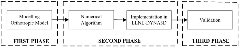
To fulfil the aim and achieve the above objectives, the research work has been divided into three phases, as depicted by Figure 1-1. The methodology used to guide this research project is concisely described in this section.

Modelling

Orthotropic Model Validation

FIRST PHASE SECOND PHASE THIRD PHASE

Implementation in LLNL-DYNA3D Numerical

[image:21.595.90.510.362.447.2]

Algorithm

Figure 1-1 Research Phases

Generally speaking, the research project consists of a mathematical formulation, algorithm implementation in DYNA3D and a validation process.

The first phase is to produce a mathematical formulation of a material model for orthotropic metals. This is a crucial step as the formulation will significantly influence the final achievement of the project.

(22)

4

capture the initial orthotropy of the orthotropic metal. This allows for stiffness matrix identification. In addition, a referential curve is used by introducing a strength model of a Mechanical Threshold Stress (MTS). Eventually, the complexity of the new constitutive model is increased by introducing an EOS.

The numerical algorithm for the new material model for orthotropic metals is structured in the second phase. At this stage, the new mathematical formulation is implemented into LLNL-DYNA3D of Cranfield University’s version. All parameters defined for the new constitutive model are defined and implemented into the DYNA3D finite element code. This requires an alteration of several routines in the code.

Eventually, the results produced by the new material model are validated against experimental data of Plate and Cylinder Impact Tests. At the end of this research project, one material model for orthotropic metals with the characteristics aimed for will be successfully implemented in the DYNA3D finite element code.

1.4 Research Scopes

The scope of this project is to examine the behaviour exhibited by orthotropic metals at finite deformation by developing a new material model developed within a consistent thermodynamic framework. The work will use a yield function analysis in order to describe the plastic deformation process for orthotropic metals.

The DYNA3D finite element code of Cranfield University’s version is selected for the implementation of the new material model, which then further used in the numerical simulation. Equally, the Truegrid and LS Prepost are adopted as a pre-processor and a post processor in this research analysis respectively.

(23)

5

addition, the MTS input parameters of the proposed material model are taken directly from Panov (2006).

1.5 Thesis Structure

Chapter 2

Literature Review

The second chapter of this thesis is a literature review related to the modelling deformation behaviour of orthotropic metals. The discussion first focuses on the conventional theory typically adopted in the formulation of materials undergoing finite deformation. The plasticity formulation of isotropic and anisotropic materials is brought to attention in this part. The formulation related to isotropic material is not complex since the continuum of the material grains collectively has no preferred direction. However, this is not the case for anisotropic-orthotropic materials.

Anisotropic materials are classified as orthotropic if they have three mutually orthogonal symmetry planes. Such materials behave in a different way and are in fact far more complex compared to isotropic materials. Due to its wide application in many fields, the deformation behaviour of orthotropic materials must be reasonably captured. Owing to the very characteristics of this material, an appropriate mathematical formulation is required, and this is the main objective of this chapter.

Chapter 3

Material Model Formulation

(24)

6

decomposition in this chapter.

Referring to the discussion in Chapter 2, Hill’s (1948) yield criterion is adopted to capture the initial yielding of material orthotropy. The main formulations and advantages of this theory are highlighted. In addition, the yield surface is assumed to maintain the initial shape as the deformation takes place. This means that the orthotropic Hill’s parameters remain constant throughout the plastic deformation. The yield function expansion is controlled by a physically based model, the Mechanical Threshold Stress (MTS) model by using isotropic hardening. This model is discussed later in this chapter.

In general, the formulations of the new material model are defined within the thermodynamics of irreversible processes due to finite deformation. The assumption of this framework is then discussed in this chapter. Since the multiplicative decomposition of the deformation gradient is adopted to be combined with the new stress tensor decomposition, the isoclinic configuration is chosen as its reference configuration where the new material model formulations are integrated. The main features related to the kinematics of this configuration are reviewed.

The new material model is defined within elastic-plastic with hardening formulations. However, such formulations obviously can be further developed to include a damage model for better accuracy. Therefore, this chapter eventually reviews the formulation of the multiplicative decomposition when damage is introduced into this framework.

Chapter 4

The New Material Model Formulation

(25)

7

are defined within an invariant theory by using the structural tensors to represent the symmetry of material orthotropy.

Since the offset of strain typically used to define the yield point (stress at which material begins to deform plastically) of metals is very small; approximately 0.2% of the strain, the formulation is limited to small elastic deformation with large rotation; hence, the Mandel stress tensor is symmetric. Hill’s yield criterion is adopted to characterise the plasticity of orthotropic materials. It can be observed that this yield criterion has been widely used in industrial simulations and provides reasonably good results as well as being numerically efficient. The expansion of the new material model yield surface (hardening part) is characterised by a referential curve of the thermally micromechanical-based model, the Mechanical Threshold Model (MTS). Generally, a finite “saturation stress”, or what can be described as a constant but small hardening rate, is achievable at finite strains of most metallic materials. The other models such as Johnson-Cook (JC) and Zerilli-Armstrong (ZA) models are unable to capture this behaviour. Moreover, the MTS model fits the experimental data more reasonably at various strains of the saturation stress.

The formulation of a multiplicative decomposition is further manipulated to formulate and integrate the proposed ‘micro-macro’ material model with respect to the isoclinic configuration. This configuration immediately eliminates the non-uniqueness of the intermediate configuration. Eventually, the complexity of the new material model is increased by combining the proposed formulations with equation of states (EOSs) to capture large deformation behaviour due to high velocity impact.

Chapter 5

The New Material Model Implementation

(26)

8

required material data and the deformation gradient tensor are available for the analysis in this subroutine.

By using the proposed formulation, a rotation tensor algorithm is developed in subroutine f3dm93 to correctly perform pull back-push forward transformations upon the related parameters between the current and the isoclinic configurations – hence, computationally inexpensive. Several theorems are required to confirm a unique rotation tensor is implemented in the LLNL-DYNA3D code. Furthermore, a new subroutine is added to examine the accuracy of the implemented rotation tensor algorithm.

To combine the new material model with the EOS (a linear polynomial and Gruneisen EOS), several subroutines in the LLNL-DYNA3D code are modified. No modification is required to change the configuration used in these subroutines to match the selected isoclinic configuration. Since the new stress tensor decomposition provides a unique alignment of pressure (new deviatoric plane) within three-dimensional stress space for orthotropic materials depending on their elastic parameters, a few alterations are required to reflect this axis direction in the combination with EOS formulation. The implementation process is finally completed by implementing the MTS model to establish the dependence of the proposed material model on strain, strain rate and temperature in relation to the isotropic hardening formulation.

Chapter 6

New Material Model Validation

(27)

9 SPCE.

The validation process is divided into two main parts. The first part, generally, is a preliminary validation process to systematically validate each part of the proposed formulations. This methodology facilitates the process to correct any error when it is found in any part of the formulations. For this purpose, three material models available in the LLNL-DYNA3D code are accordingly adopted; Material Types 10, 22 and 33. These material models are used to validate the elastic isotropy, the elastic orthotropy and the elastic-plastic formulations, respectively. This preliminary part of the validation process is finalised by examining the strain rate and temperature sensitivity of the proposed material model.

The validation process is continued with a comparison between the proposed material model against the experimental test data. The accuracy of the proposed material model to represent the deformation behaviour of Aluminium 7010-T6 in a Plate Impact test and Taylor Cylinder Impact test is deeply scrutinised at this validation stage. The finite element (FE) models are specifically simulated to appropriately represent these impact cases. Three different impact velocities in longitudinal and transverse direction are simulated for the Plate Impact test:

_{. Eventually, the Taylor Cylinder impact tests are modelled in}

three-dimensional stress state with and impact velocities. The results produced by the new material model are compared with the experimental data in terms of the final radius and length of the deformed cylinder.

Chapter 7

Conclusion

(28)

10

increase the accuracy of the new material model is proposed at the end of this chapter.

1.6 Notation

Three different notations are used throughout this thesis: indicial, tensor and matrix. These notations are adopted in equations relating to continuum mechanics and finite element implementation. Even though different notations are being adopted, the researcher has, however, tried to minimise the variety of notations and remain consistent in the formulations.

1.6.1 Indicial Notation

Generally, in indicial notation, the components of matrices and tensors are clearly specified. For example, any vector which is categorised as a first-order tensor is denoted by , where the range of the index represents the number of dimensions. Indices repeated twice in a term are actually summed. In three dimensions for instance, suppose is the position vector with magnitude , then

_{Equation 1-1}

The second expression in Equation 1-1 shows that , , . It should be borne in mind that it is almost impossible to avoid indicial notation in the implementation of FE methods.

1.6.2 Tensor Notation

(29)

11

employs this notation. Using tensor notation, first-order tensors or greater are indicated in boldface. Lower case boldface letters are normally used for first-order tensors; upper boldface letters meanwhile are adopted for higher order tensors.

Equation 1-1 is rewritten in tensor notation as , where a dot in this expression denotes a contraction of the inner indices. Strictly speaking, the tensors on the right hand side (RHD) have only one index; hence, the contraction applies on those indices. The major exception is however applied for the Cauchy stress tensor , which is expressed by a lower case boldface letter.

Tensor expressions are distinguished from matrix expressions via dots and colons between terms, as demonstrated by the linear constitutive equation below.

⏟

Equation 1-2

1.6.3 Matrix Notation

Matrix notation is usually used in the implementation of FE methods. In this thesis, matrix notation holds the same expression as for tensor notation, but no connectivity symbols are included. Therefore, Equation 1-1 can be expressed as .

First-order tensors are denoted by lower case boldface letters. A vector such as velocity can be written as , and considered column matrices are as follows:

{ } Equation 1-3

(30)

12

[

]

Equation 1-4

To describe those notations used in this thesis, the quadratic form of is given as follows:

⏟

Equation 1-5

(31)

13

Chapter 2

Literature Review

T

his chapter provides a literature review related to the modelling deformation

behaviour of orthotropic metals. The chapter starts with a discussion of the fundamental theory associated with the plasticity of isotropic and orthotropic materials. This is followed by discussing the most suitable decompositions for the formulation of orthotropic metals. Accordingly, the chapter then considers in detail the formulation of multiplicative decomposition of the deformation gradient . Finally, this chapter briefly introduces the structural tensors used to track the evolution of the principal directions of material orthotropy.

2.1 Insight into Plasticity

(32)

14

This approximation replaces a large number of particles by a few quantities. In other words, this theory replaces the particles with a continuous medium that is characterised by several field quantities associated with material internal structure, such as temperature and density.

2.2 Isotropic Plasticity

In the theory of plasticity, the behaviour of materials undergoing plastic deformation is well described with a yield function (yield surface), a flow rule and a hardening law. Yield surface is assumed to represent a plastic potential for the case of associative plasticity where the associated flow or normality rule applies. The plastic potential is defined as a stress at which yielding occurs for a given stress state. The gradient (the normal to the yield surface at the loading point) gives the direction of the plastic strain rate. Equally, a yield surface represents the limitation of the elastic regime of any material and determines the point at which the material starts to yield.

The flow rule meanwhile identifies the correlation between the deviator stress and the strain rate tensor.

The determination of the plastic stress-strain relationship for plastic deformation was originated by Saint Venant in 1870. He suggested that the principal axes of the strain increment coincided with the axes of the principal stresses. In addition, a relationship between the ratios of the components of the strain increment and the ratio of the stresses was originally proposed by Levy in 1871 and independently reasserted by von Mises in 1913 when the relationship became better known (Slater, 1977). These equations are usually known as the Levy-Mises equations. The Levy-Mises theory is based on the following assumptions

 The elastic strain is small, hence it can be neglected

(33)

15

hence is coaxial with . Consequently, the equation of this theory can be expressed by

Equation 2-1

where or ̇ is a scalar non-negative proportionality factor which is not constant and may vary throughout the stress history. The parameter ̇ is determined from the yield criterion.

In contrast, when the elastic strain is comparable to that of the plastic strain , it may not be neglected. The stress-strain relations for elastic-perfectly plastic material were first proposed by Prandtl in 1924 and generalised independently by Reuss in 1930. Plastic deformation is assumed to be isochoric, while elastic deformation causes volume changes as well as shape changes.

Normally during metal-forming processes, the elastic incremental strains are negligible compared to the plastic incremental strains within the fully developed plastic region. Hence it is possible to neglect the elastic contribution as being insignificant.

When dealing with elastoplastic deformation, however, where the elastic component of the total incremental strain is of importance, it is necessary to resort to the Prandtl-Reuss assumption. Conversely, if the elastic incremental strain is neglected then the material is considered as rigid-perfectly plastic. This condition is compatible with the Levy-Mises assumption. It is assumed that no strain occurs until deformation reaches the yield stress of the body and the total strain increment is identical to the plastic strain increment. This formulation is useful in obtaining plastic deformation for most metals where the plastic strain is much larger than the elastic strain , (Khan and Huang, 1995).

(34)

16

through an elastic potential function, the complementary elastic strain energy , such that

Equation 2-2

By generalizing and applying this idea to plasticity theory, Mises proposed there existed a plastic potential function ( ) and the plastic strain rate ̇ . This assumption can be written as

̇ ̇ ( ) Equation 2-3

In this equation, the yield criterion can be used to determine ̇. The plasticity theory that is based on a flow rule assumption is called a plasticity potential theory. The key aim of this theory is to define the plastic potential, ( ). A common approach adopted in the associative plasticity theory is to assume that the plastic potential function ( ) is identical to the yield function ( ).

( ) ( ) Equation 2-4

Thus Equation 2-3 can be re-expressed by

̇ ̇ ( ) Equation 2-5

where the plastic strain rate, ̇ is defined as normal to the yield surface. This condition is called an associated flow rule. Conversely, the flow rule is non-associated if ( ) ( ). Experimental observations prove that the plastic deformation of metals can be represented by the associated flow rule.

(35)

17

̅ ∫ ̅ _{Equation 2-6}

Equation 2-6 states the amount of hardening depends only on the effective plastic strain and is called the plastic strain hardening hypothesis. The second hypothesis is proposed by Hill (1948) and states that the degree of hardening depends only on the total plastic work done, . Applying this condition for isotropic materials gives

∫ _{Equation 2-7}

The evolution of the yield surface can be isotropic, anisotropic, or a combination of the two, regardless of the initial shape of the yield surface. The isotropic hardening allows for expansion of the yield surface without any distortion as described in Figure 2-1.

A yield function for isotropic and pressure-insensitive materials can be expressed in terms of isotropic hardening as follows:

( ) ( ) _{Equation 2-8}

[image:35.595.166.441.378.565.2]

where and represent the second and third invariants of the deviatoric stress . It can be observed from Equation 2-8 that only one hardening parameter is required to

(36)

18

the radius of the yield surface. The evolution of then can be written as

̅ _{Equation 2-9}

Equation 2-9 confirms the evolution of the radius of the yield surface, therefore is proportional to the measure of plastic deformation.

On the other hand, the kinematic hardening was motivated by the Bauschinger effect in the uniaxial tension-compression. In fact, it is compatible in the case of cyclic loading. The concept involved in this hardening rule is to observe the centre of the yield surface, as shown in Figure 2-2.

In the kinematic hardening model, an internal variable called the backstress is introduced. It is used to define the position of the yield surface centre in the stress space and changes due to plastic strain hardening. Suppose that the initial yield surface is described by

[image:36.595.137.462.350.538.2]

(37)

19

surface during the plastic loading as follows:

( ) ( ) _{Equation 2-11}

In addition, an equation of state (EOS) is required in modelling a material that involves very high pressures and shockwaves. Meanwhile, the previous concepts are combined with a consistency condition ̇ in identifying the relationship between stress and strain in the elastic and plastic regimes. The behaviour of metals at a continuum scale within elastic and plastic regimes can also be described using damage and failure models.

2.3 Anisotropic Plasticity

It can be observed that so far the theory related to isotropic materials is not very complex. It may therefore undergo rotations without affecting the material response. However, this is not the case for anisotropic materials. The mechanical properties that affect the yield surface will start to change (be distorted) when material undergoing plastic deformation starts to rotate. Therefore, a set of variables normally has to be introduced to take into account the evolution and orientation of such materials.

Generally speaking, anisotropic materials exhibit different mechanical properties in different directions which can be specified by magnitude and orientation. Elastic anisotropy has an influence on the initial yield surface shape.

(38)

20

2.3.1 Yield Criteria

A homogeneous yield function of degree two which is used to model an orthotropic plastic response of rolled sheet was first proposed by Hill (1948). This concept can be regarded as a solid foundation for the subject in the case of metals. In the literature, numerous researchers have tried to investigate and examine the validity of this basic framework. The consensus is that the proposed model is too flexible and only well-suited to certain metals, summarised by Hosford (1988).

In addition to Hill’s yield function, various types of yield function have been constructed in the literature. For the sake of simplicity, only a few of them are briefly highlighted and grouped in this section, and a general comment is made accordingly.

The yield criteria modelled for metals can be found in Barlat and Lian (1989), Hill (1990, 1993), Cazacu et al. (2006), Banabic et al. (2000) and others. The yield functions proposed in Barlat and Lian (1989) and Hill (1990) are modelled for metals that are subjected to plane stress condition.

The yield criteria proposed particularly for aluminium alloy sheets can be found in Barlat et al. (1991, 1997), Karafillis and Boyce (1993) and in Cazacu and Barlat (2003). Further, Barlat and his group have proposed yield functions of the order in Barlat and Lian (1989) and Barlat et al. (1991, 1997). Constitutive models that are consistent with a micromechanical crystallographic-based yield criteria can be observed in Barlat and Lian (1989) and Barlat et al. (1991). In addition, a linear transformation-based anisotropic yield function can be found in Barlat et al. (2005), Plunkett et al. (2006, 2007) and others. Several non-quadratic yield criteria have been proposed by Gotoh (1977), Hill (1979), Logan and Hosford (1980) and others.

(39)

21

the case where the loadings are not co-linear with the anisotropic axes.

In addition, a few researchers such as Feigenbaum, Dafalias, Voyiadjis and Tatten have concentrated on distortional hardening as a consequence of internal variables’ evolution, (Dafalias, 2000; Feigenbum and Dafalias, 2007, 2008). To track the results provided for these models, we may refer to Feigenbum and Dafalias (2007). Generally this approach results in complexity of the model since more constants were introduced to describe the distortional hardening. However the model as a whole has shown a capability to capture distortion of the yield surface for different loading paths and metals.

On the other hand, most of the micromechanical based yield criteria can provide the required results. However they are not simple enough for fast numerical applications (Chung and Shah, 1992).

Some of the above yield criteria have been successfully implemented into finite element FE codes in order to model sheet metal forming processes as discussed in Chung and Shah (1992), Tugcu and Neale (1999), Inal et al. (2000), Worswick and Finn (2000) and others. A few of them are discussed in this section.

For instance, Chung and Shah (1992) have investigated Barlat’s six components anisotropic yield function as proposed in Barlat et al. (1991) by modelling hydraulic bulge and cup drawing tests in ABAQUS. The same yield criterion has also been examined in Inal et al. (2000) to investigate earing phenomena in the deep drawing of rolled aluminium sheets.

(40)

22

by Worswick and Finn (2000) by simulating a stretch flange forming operation. The results obtained in the chosen numerical simulations show good agreement. This proves that these yield criteria are capable of simulating the forming processes. However, there are still theoretical problems: specifically the issues related to the rotation and distortion of the initial anisotropic reference frame (Tugcu and Neale, 1999). A rigorous review and comments on the yield criteria proposed to capture the anisotropy of sheet metals can be found in Banabic et al. (2010).

2.4 Decompositions for Orthotropic Materials

Anisotropic materials are classified as orthotropic if they have three mutually orthogonal symmetry planes. In many engineering components, the orthotropy is induced by a number of manufacturing processes such as rolling and stamping etc. Composites are also examples of orthotropic materials. In fact, most elastoplastic materials exhibit anisotropic behaviour due to their structure orientation and evolution (Eidel and Gruttmann, 2003).

The constitutive equation based on additive decomposition of generalised strain measures is basically not suitable for the modelling of orthotropic materials’ behaviour. As demonstrated by Itskov (2004), this kind of constitutive model leads to spurious shear stresses which are independent of the elastic material properties for orthotropic materials.

(41)

23

gradient provides a natural framework for the frame-invariant description of anisotropic elasticity and anisotropic plastic yield (Belytschko et al., 2000).

An additive decomposition of strain and strain rate has been found satisfactory for the case of infinitesimal rotations and for uniaxial (non-rotational) deformations (Reinhardt and Dubey, 1998). However, such decomposition is not applicable when material is undergoing finite rotations.

To conclude, it is important to use a multiplicative decomposition of deformation gradient instead of using an additive decomposition of generalised strain measure in modelling a behaviour model of orthotropic metals.

2.5 Multiplicative Decomposition

At the very beginning, it is worth recollecting that the analysis is performed within a macroscopic scale where the system is typically well described by a continuum approach which leads to the continuum theory.

Suppose we have a body , filled with solid continuum and deforming in time for body material points which can be identified by . Also it should be mentioned here that a material point represents a large number of molecules and their corresponding behaviour in order to maintain generality and make the consideration applicable for arbitrary deformations.

(42)

24

Configuration is the undeformed configuration of the deformable body at time . is the current deformed configuration at time . Furthermore, assuming a smooth deformation regardless of the cause of deformation, one can consider to be the deformation gradient of one-to-one mapping of an infinitesimal material element from

in to in such that

_{Equation 2-12}

A fixed set of Cartesian coordinate axes is used for both the initial and current configurations. The plastic intermediate configuration ̅ is obtained by elastically distressing (unloading) the current configuration to zero stress. This configuration

̅ _{differs from the initial configuration} _{by plastic deformation, and differs from}

the current configuration by elastic deformation. Let be the material element in

̅ _{, then we get}

_{Equation 2-13}

𝛀̅_𝑝 (Vi u l onfigu ion) 𝛀

𝛀

𝐅𝑝 𝐅_𝑒

𝐱_𝑝

𝐱 𝐗

[image:42.595.125.456.92.313.2]

𝐅

Figure 2-3 Decomposition of decomposition gradient and definition of intermediate

(43)

223

References

1948 Hill, R., A theory of the yielding and plastic flow of anisotropic metals. Proc. Roy. Soc. 193 Ser. A, 281-297

1950 Hill, R., Mathematical Theory of Plasticity. Clarendon Press, Oxford

1969 Jaeger, J.C., Cook, N. G. W., Fundamentals of rock mechanics: Barnes and Noble, New York, N.Y. and Methuen, London, 513 pp., 120s

1969 Lee, E. H., Elastic-plastic deformation at finite strains. ASME Trans. J. Appl. Mech., 36, 1

1969 Malvern, L. E., Introduction to the Mechanics of a Continuous Medium, Prentice-Hall Inc

1970 Spencer, A. J. M., On generating functions for the number invariants of orthogonal tensors, Mathematika, 17, 275-286

1971 Spencer, A. J. M., Theory of invariants, In continuum physics, Academic Press, New York, 239-353

1972 Mandel, J., Plasticité Classique et Viscoplastié, CISM lecture Notes, Springer-Verlag, Wien

1973 Mandel, J., Equations constitutives et directeurs dans les milieux plastiques. Int. J. Solids Structures, 9, 725

1977 Boehler, J. P., On irreducible representations for isotropic scalar functions, ZAMM 57, 323-327

1977 Gotoh, M., A theory of plastic anisotropy based on a yield function of fourth order (plane stress state)—I/II. Int. J. Mech. Sci. 19, 505-512, 513-520

1977 Slater, R.A.C., Engineering Plasticity, Theory and Application to Metal Forming Process, The Macmillan Press LTD, London and Basingtoke

1978 Boehler, J. P., Lois de comportement anisotrope des milieux continus, J. Mec, 17, 153-190

1979 Hill, R., Theoretical plasticity of textured aggregates. Math. Proc. Camb. Phil. Soc. 85, 179-191

(44)

224

calculations assuming (111)-pencil glide, Int. J. Mech. Sci., 22, 419

1983 Hallquist, J., Theoretical manual for DYNA3D, Technical report, Lawrence Livermore National Laboratory

1984 Rosenberg, Z., Mayseless, M., Partom, Y., The use of Manganin stress transducers in impulsively loaded long rod experiments. J. Applied Physics, 51, 202-204

1985 Callen, H. B., Thermodynamics and an introduction to thermostatistics. Wiley, New York

1985 Dafalias, Y. F., The plastic spin, J. Appl. Mech., 52, 865-871

1985 Johnson, G. R., Cook, W. H., Fracture characteristics of three metals subjected to various strains, strain rates, temperatures and pressures, Engineering Fracture Mechanics, 21(1), 31-48

1987 Barlat, F., Crystallographic texture, anisotropic yield surface and forming limits of sheet metals. Mat. Sci. Eng., 91, 55

1987 Dafalias, Y. F., Issues on the constitutive formulation at large elastoplastic deformations, Part 1: Kinematics. Acta Mechanica, 69, 119-138

1987 Zerilli, F.J., Armstrong, R.W., Dislocation-mechanics-based constitutive relations for material dynamics calculations, J. Appl. Phys., Vol. 61, N0.5, 1987, pp. 1816-1825

1988 Follansbee, P.S., Kocks, U.F. A constitutive description of the deformation of copper based on the use of the mechanical threshold stress as internal state variable. Acta Metallurgica, 36, 81-93

1988 Hosford, W.F., Limitations of Non-Quadratic Anisotropic Yield Criteria and Their Use in Anal-ysis of Sheet Forming, In International Deep Drawing Research Group (ed.), Controlling Sheet Metal Forming Processes, ASM International, 163-170

1989 Barlat, F., Lian, J. Plastic behaviour and stretchability of sheet metals. Part I: a yield function for orthotropic sheets under plane stress conditions. Int. J. Plasticity 5, 51-66

1989 House, J. W., Taylor impact testing. Final Report for Period June 1987-January 1989, University of Kentucky, Lexington, Kentucky

1990 Hill, R., Constitutive modelling of orthotropic plasticity in sheet metals. J. Mech. Phys. Solids 38 (3), 405-417

(45)

225

materials. Int. J. Plasticity 7, 693-712

1992 Chung, K., Shah, K., Finite element simulation of sheet forming for planar anisotropic metals. Int.J. Plasticity 8, 453-476

1993 Hill, R., A user friendly theory of orthotropic plasticity in sheet metals. Int. J. Mech. Sci. 35 (1), 19-25

1993 Karafillis, A.P., Boyce, M.C., A general anisotropic yield criterion using bounds and a transformation weighting tensor. J. Mech. Phys. Solids 41, 1859–1886

1994 Aravas, N., Finite-strain anisotropic plasticity and the plastic spin. Modelling Simul. Mater. Sci. 2, 483-504

1994 Hansen, N. R., Schreyer, H. L. A thermodynamically consistent framework for theories for elastoplasticity coupled with damage. Int. J. Solid Structures 31 (3), 359-389

1994 Zheng, Q. S., Theory of representations for tensor functions-A unified invariant approach to constitutive equations. Applied Mechanics Reviews 47 (11), 545

1995 Khan, A. S., Huang, S. Continuum Theory of Plasticity, John Wiley & Sons Inc, New York

1995 Lubarda, V. A. and Krajcinovic, D. Some Fundamental Issues in the Rate Theory of Damage-Elastoplasticity, Int. J. Plasticity, 11, 763-797

1997 Barlat, F., Maeda, Y., Chung, K., Yanagawa, M., Brem, J., Hayashida, Y., Lege, D., Matsui, K., Murtha, S., Hattori, S., Becker, R., Makosey, S., Yield function development for aluminium alloy sheet. J. Mech. Phys. Solids 45, 1727

1997 Kim, K. H., Yin, J. J., Evolution of anisotropy under plane stress. Journal of the Mechanics and Physics of Solids 45, 841-851

1998 Campbell, J., Lagrangian hydrocode modeling of hypervelocity impact on spacecraft, PhD Thesis, Cranfield University, Cranfield, UK

1998 Reinhardt, W. D., Dubey, R. N., An Eulerian-based approach to elastic-plastic decomposition. Acta Mechanica 131, 111-119

(46)

226

the Taylor cylinder impact test for orthotropic textured materials: experiments and simulations. International Journal of Plasticity 15, 139-166

1999 Tugcu, P., Neale, K.W., On the implementation of anisotropic yield functions into finite strain problems of sheet metal forming. International Journal of Plasticity 16, 701-720

2000 Banabic, D., Bunge, H. J., Pohlandt, K., Tekkaya, A. E., Formability of metallic materials, Springer Heidelberg

2000 Belytschko, T., Liu, W. K., Moran, B., Nonlinear Finite Elements for Continua and Structures, John Wiley & Sons Ltd, Chichester

2000 Dafalias, Y.F, Orientational evolution of plastic orthotropy in sheet metals. J. Mech. Phys. Solids 48, 2231-2255

2000 Inal, K., Wu, P.D., Neale, K.W., Simulation of earing in textured aluminum sheets. Int. J. Plasticity 16, 635-648

2000 Worswick, M.J., Finn, M.J., The numerical simulation of stretch flange forming. Int. J. Plasticity 16, 701-720

2001 Hanson, K. M., Hemez, F. M., A framework for assessing confidence in Computational predictions. Exper. Techniques, 25, 50-55

2002 Brannon, R. M., Rotation: A review of useful theorems involving proper orthogonal matrices referenced to three dimensional physical space, Computational Physics and Mechanics, Sandia National Laboratories, Albuquerque

2002 Lubarda, V.A., Elastoplasticity Theory, CRC Press LLC, Corporate Blvd., Boca Raton, Florida

2002 Miehe, C., Apel, N., Lambrecht, M., Anisotropic additive plasticity in the logarithmic strain space: modular kinematic formulation and implementation based on incremental minimization principles for standard materials. Comput. Methods Appl. Mech. Engrg. 191, 5383-5425

2002 Schröder, J., Gruttmann, F., Löblein, J., A simple orthotropic finite elasto– plasticity model based on generalized stress–strain measures. Computational Mechanics, 30, 48–64

2003 Banabic, D., Kuwabara, T., Balan, T., Comsa, D.S, Julean, D., Non-Quadratic Yield Criterion for Orthotropic Sheet Metals Under Plane-Stress Conditions, Journal of Mechanical Sciences July, 45, 797-811

(47)

227

yielding of anisotropic aluminium alloys. Int. J. Eng. Sci. 41, 1367–1385 2003 De Vuyst, T., Hydrocode modelling of water impact, PhD Thesis, Cranfield

University, Cranfield, UK

2003 Eidel, B., Gruttmann, F., Elastoplastic orthotropy at finite strains: multiplicative formulation and numerical implementation. Computational Materials Science 28, 732-742

2003 Farnsworth, G. V., Robinson, A. C., Improved Kinematic Options in ALEGRA, Sand Report, SAND2003-4510, Sandia National Laboratories, Albuquerque

2003 Krüger, L., Meyer, L.W., Razorenov, S.W., Kanel, G.I. Investigation of dynamic flow and strength properties of Ti6-22-22S at normal and elevated temperatures. Int. J. Impact Eng., 28 (8), 877-890

2003 Rajendran, A.M., Critical measurements for validation of constitutive equations under shock and impact loading conditions. Optics and Lasers in Engineering, 40, 249-262

2003 Sansour, C., Bocko, J., On the numerical implications of multiplicative inelasticity with an anisotropic elastic constitutive law. Int. J. Numer. Meth. Engng, 58, 2131-2160

2004 Itskov, M., On the application of the additive decomposition of generalized strain measures in large strain plasticity. Mech. Res. Commun. 31, 507-517 2004 Itskov, M., Aksel, N., A constitutive model for orthotropic elasto-plasticity at

large strains. Archive of Applied Mechanics 74, 75-91

2004 Lin, J. I., DYNA3D: A Nonlinear, Explicit, Three-Dimensional Finite Element Code for Solid and Structural Mechanics User Manual, Lawrence Livermore National Laboratory

2004 Miehe, C., Apel, N., Anisotropic elastic–plastic analysis of shells at large strains. A comparison of multiplicative and additive approaches to enhanced finite element design and constitutive modelling. Int. J. Numer. Meth. Engng, 61, 2067-2113

2005 Barlat, F., Aretz H., Yoon J.W., Karabin, M.E., Brem, J.C., Dick, R.E., Linear transformation based anisotropic yield functions, International Journal of Plasticity 21, 1009-1039

2005 Voyiadjis, G. Z., Kattan, P. I., Damages mechanics, Taylor and Francis Group 2006 Cazacu, O., Plunkett, B., Barlat, F., Orthotropic yield criterion for hexagonal

Modelling rate dependent behaviour of orthotropic metals

SCHOOL OF ENGINEERING

PhD THESIS

Academic Year 2011/2012

MOHD KHIR MOHD NOR

MODELLING RATE DEPENDENT BEHAVIOUR OF

ORTHOTROPIC METALS

Supervisor:

This thesis is submitted in partial fulfilment of the requirements

for the degree of PhD

ABSTRACT

TABLE OF CONTENTS

TABLE OF FIGURES

TABLE OF TABLES

NOMENCLATURES

Chapter 1

Introduction

T

1.1

Research Background

1.2

Aim and Objectives

1.3

Research Methodology

1.4

Research Scopes

1.5

Thesis Structure

1.6

Notation

Chapter 2

Literature Review

T

2.1

Insight into Plasticity

2.2

Isotropic Plasticity

2.3

Anisotropic Plasticity

2.4

Decompositions for Orthotropic Materials

2.5

Multiplicative Decomposition

References