The fractional calculus numerical algorithms and its application to the viscoelastic material problem

Journal of Chemical and Pharmaceutical Research, 2013, 5(12):821-828

Research Article

_{CODEN(USA) : JCPRC5}

ISSN : 0975-7384

The fractional calculus numerical algorithms and its application to the

viscoelastic material problem

Ai-Min Yang

1,2*

, Ling Zhang

1

, Xiao-Jun Men

1

, Yi-Jun Zhou

3

and Ying Jiao

3

1

College of Science, Hebei United University, Tangshan, China

2

College of Mechanical Engineering, Yanshan University, Qinhuangdao, China

3

Qinggong College, Hebei United University, Tangshan, China

_____________________________________________________________________________________________

ABSTRACT

This paper studied the fractional calculus, given three types of numerical methods of solving fractional differential equations, that is the Fractional Euler method, The Fractional Backward differential method(BDF method) and the Fractional Order Reduced Backward differential method(FORBDF method). The numerical results show that these methods are effective, and we discussed the application of the fractional calculus to the viscoelastic material problem. Finally, the paper made a summary of the major work and prospected for future work.

Key words: Fractional calculus, Euler method, BDF method, FORBDF method, viscoelastic material

_____________________________________________________________________________________________

INTRODUCTION

The development history of researches on fractional calculus and its theory is almost as old as the integer-order calculus. The concept of fractional calculus first appeared in Leibniz’s diary in the September 30, 1695, he discussed the 0.5-order calculus and the significance of fractional derivatives, in which marks the theory sprout. However only after 124 years later that is in 1819 LA Croix first put forward a result of the simplest fractional

derivative:

1/2 1/2

2

x x

α

α = π

Over the next few centuries, N. H. Abel [1], J. Liouville [2], B. Riemann, A. K. Grunwald, A. V. Letnikov, H. Weyl [3], A. Marehaud, H. T. Davis, A. Erdelyi, M. Resz, C. Fox and many other scientists conducted in-depth research for fractional calculus , and made important contributions to the development of fractional calculus. The fractional calculus theory increasingly perfect in Euclidean measure, But mainly as a pure theoretical field of mathematics useful only for mathematicians, Because of lacking for boost of actual application background, the theory of fractional calculus developed very slowly [4-7].

structure, all this have aroused great concern of scholars at home and abroad.

In July, 1974, B. Ross organized the first fractional differential operators meeting in New Haven University, and edited session record. In 1965, K. B. Oldhamand J. Spanier [9] studied the fractional differential operator and published the first monograph in 1974, that is the fractional calculus, and there is also a thematic journal that is the journal of rational calculus, then also appeared the monograph on fractional differential operator, for example, Me Bride(1979), Samko, Kilbas and Mariellev (1987-1993), Nishimoto(1991), Miller Ross(1993),Rubin(1996), kiryanova(1994) and Podlub (1999). Some treatise studied the applications in mathematics in physics of fractional differential theory, for example, Davis, shilov, Dzherbashian, Caputo, Babenko, Gorenflo and so on .

The numerical methods for fractional differential equations [6] have been heated discussion in domestic and foreign recently, including time and space fractional derivative, single and multi-fractional derivative [7-8], fractional ordinary differential equations and fractional partial differential equations. In 1986, Lubich first extended the BDF method to the numerical calculation of fractional integration and differentiation, and received a fractional approximation scheme of the BDF. In 1997, K. Diethie constructed a numerical method based on integral equation for the fractional differential equation of linear problem, and accessed its local and global error. In the same year, K.DiethalmandG.Walzln8 proposed the extrapolation method to solve fractional differential equations in order to improve the accuracy of numerical methods. 2001, N. J. Ford and C. Simpson analyzed the fixed storage guidelines to the nonlinear fractional differential and proposed nested grid programs to achieve variable step calculations method in order to obtain a better solution reasonable approximation. From 2002 to 2005, K. Diethelm proposed the fractional Admas method, the fractional estimate correction method, and gives the error analysis and the program for numerical methods. In 2003, Cuesta solves differential equations of fractional integral fractional Trapezoidal formula in Banach space. In China, Lin Ran and Liu Fawang studied the method of solving linear ordinary differential equations using BDF method and proved its compatibility, convergence and stability. Liu fawang construct the corresponding numerical methods for several different types of fractional differential equations[9-12] For example, the fractional relaxation equations, the fractional Bagley-Torvik equation, the fractional relaxation -Osciliation equation, the time fractional diffusion-reaction equations and control system of fractional differential equations, and gives its numerical methods convergence and stability analysis using fractional dispersion coefficient characteristics. Cao Xuenian and K.Burrag put forward the idea of nesting methods, which obtain effective adjustable step size implementation and conducted numerical stability analysis and obtain stability region.

About the research of the fractional differential equations and numerical methods, F. Mainardi and R. Gorenflo developed the fractional calculation model, and obtained fractional basic solution of partial differential equations through Laplace transform, Fourier transform, Mellin transform. Mark Meerschaert studied the numerical methods of fractional-order partial differential equations, including linear method, finite difference method (explicit, implicit, extrapolation and so on), the finite element method and the infinite element method, etc. Sanz -Serna, Chen Chuansen, Thomee, Wahlbin, Huang Yunqing, XU large Liufa Wang and others made a good job in this field, they get the new numerical methods and techniques and theoretical analysis solution of partial differential equations.

DEFINITION OF FRACTIONAL CALCULUS

The definition of fractional derivative have many forms, and the ordinary defined is

Riemann

−

Liouville

,

Gruwald



−

Letnikov

_and

Caputo

_[13].

Definition 1 The

Gruwald



−

Letnikov

fractional derivative：

( )

[ ]/

( )

(

)

0 0

lim

1

,

0

1

j t h G

O t

h

j

D y t

h

y t

jh

n

n

j

α −α

α

_α

→ ₌

 

=

−

_{ }

−

≤ − < ≤

 

∑

(1)

where

Γ

( )

z

is the

Gamma

function, and the form is defined as：

( )

1

0

t z

z

∞ − −

e t

dt

Γ

=

_∫

______________________________________________________________________________

( )

₍

₎

( )

0

1

,

0

1

0

(

)

n t a

t

R

d

y

D y t

d

n

n

n a

dt

t

t

t

α

t





=

_

_

≤ − < <

Γ −





∫

−

₍₂₎

where

Γ

( )

z

is

Gamma

function, and the form is defined as：

( )

1

0

t z

z

∞ − −

e t

dt

Γ

=

∫

(3)

when

α = ∈

n

N

, it satisfy:

( )

n

( )

R

O t n

d

D y t

f t

dt

α

₌

Definition 3 The

Caputo

fractional derivative[14]：

( )

(

)

( )

_{( )}

(

)

( )

1 0

1

,

0

1

,

,

.

n t n C O t n n

y

d

n

n

n

t

D y t

d

f t

if

n

N

dt

α α

t

t

α

α

t

α

+ −



≤ − < <



Γ

−



−

= 



= ∈



∫

(4)

it satisfies

(

)

( )

_{( )}

(

)

1

( )

0

1

lim

.

n _n t n n n

y

d

d

f t

n

t

α

dt

α

t

t

α

_t

+ −

→

Γ

−

∫

₋

=

The three definition of fractional have the following relationships：

(1) If

y t

( )

is continuously differentiable of order

n

−

1

during, and interblend then for any 0< <α n Riemann, −Liouville _{fractional derivative and}

Gruwald



−

Letnikov

_{fractional derivative is}

equivalent, and if

0

≤ − ≤ < ≤

m

1

α

m

n

,

then

0

< <

t

T

have the following relationship:

( )

( )

1

₍

( )

₎

₍

_{) (}

)

1

( )

0 0 0 0

0

1

1

k k

m _t m

R G m

t t

k

t

y

D y t

D y t

t

y

d

k

m

α _α

α α

_t

_{t t}

α

α

−

− − −

=

=

=

+

−

Γ − +

Γ

−

∑

∫

(5)

(2)The relationship of

Riemann

−

Liouville

fractional derivative and

Caputo

fractional derivative is：

( )

1

₍

( )

₎

0 0 0

0

1

k k m R k

t

y

D y t

k

α α

α

− − =

+

Γ − +

∑

(6) Among them,

n

− < <

1

α

n

.

The mathematical model is different of the fractional differential equations as the different background of the issue; the research about fractional ordinary differential equations numerical methods, the currently studied fractional differential equations is the follow one:

( )

(

( )

)

( )

( )

, 0 k m D y tα f t y t t T

 = < ≤

 

= ∈

When

n

− ≤ <

1

α

n

, the

D y

α

is the

Riemann

−

Liouville

rational derivative for

y

or

Caputo

rational derivative.

THE NUMERICAL METHODS

Considering the following initial value problem of fractional differential equation:

1

0 0

( )

( ( ))

( ( ))0

(0)

m

y t

D

f y t

g y t

t

y

y y

R

α −

′



=

+

< ≤ Τ



∈



₍₈₎

Where

1

1,

D

α

f

α

−

< ≤

0

_{is the Riemann-Liouville fractional derivative of}

f

_{, the form is defined as follow:}

1 1

0

( )

d

t

D

f t

e t

dt

dt

α α

α

∞

−

₌

− −

Γ

∫

1

（）

(9)

Where

Γ

（）

α

is Gamma function, which is defined as follow:

1

t

e t

α

dt

α

∞ − −

Γ

=

∫

0

（）

Solving the first equations of the above-mentioned, we give several numerical methods solve fractional differential equations; they are fractional Euler method, the fractional backward differential equation and the reduced order of fractional backward differential equation.

The Euler method: The Euler method is the easiest numerical method to solve fractional ordinary differential equations, the basic format is:

1

1

(

)

(

)

a

n n n n

y

₊

=

y

+

hD

−

f y

+

hg y

(10) We need the numerical approximation scheme of the fractional derivative in order to achieve the above numerical method, here we use modified form which proposed by Diethelm, this leads to the following approximation:

1 1

0

(

)

(

)

(1

)

n

n jn j

j

h

D

f y

C f y

α α

α

− −

=

≈

Γ +

∑

(11)

Where

h

n

Τ

=

the size of integration step is,

t

j

=

jh j

,

=

0,1, 2,

2

, ,

n y

n is the approximation of exact solution

y t

( )

n _{, the coefficient}

C

jn

,

j

=

0,1,

2

, ,

n

determined by the following relationship:

1

(

1) ;

0;

(

1)

2(

)

(

1) :

1, 2,

,

1;

1, 2,

,

1

1;

;

jn

n

n

n

j

C

n

j

n

j

n

j

j

n

j

n

j

n

α α α

α α α

α

−



−

+ −

=



=

_

− +

−

−

+ − −

=

−

=

−



₌



2

2

(12) Generally speaking, the approximation order of formula (4) is

1

(

).

O h

+α

Fractional Backward differential Formula: The numerical value of Fractional Backward differential Formula is:

1

0

(

)

(

)

k

j n j n k n k j

y

hD

α

f y

hg y

α

−

+ + +

=

=

+

∑

______________________________________________________________________________

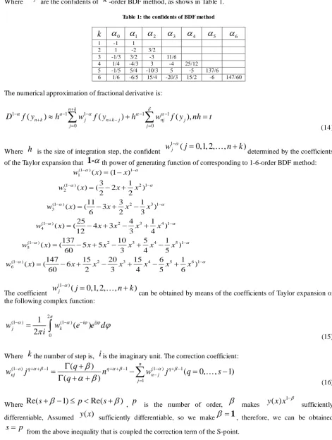
[image:5.595.66.538.85.710.2]

Where

α

j _{are the confidents of}

k

_{-order BDF method, as shows in Table 1.}

Table 1: the confidents of BDF method

k

α

0

α

1

α

2

α

3

α

4

α

5

α

6

1 -1 1 2 1 -2 3/2 3 -1/3 3/2 -3 11/6 4 1/4 -4/3 3 -4 25/12 5 -1/5 5/4 -10/3 5 -5 137/6 6 1/6 -6/5 15/4 -20/3 15/2 -6 147/60

The numerical approximation of fractional derivative is:

1 1 1 1 1

0 0

(

)

(

)

(

),

n k a

n k j n k j nj j

j j

D

f y

h

w

f y

h

w

f y

nh

t

δ

α + α α α

− − − − −

+ + −

= =

≈

∑

+

∑

=

(14)

Where

h

is the size of integration step, the confident

1

(

0,1, 2,

,

)

j

w

−α

j

=

2

n

+

k

determined by the coefficients of the Taylor expansion that

1-

α

th power of generating function of corresponding to 1-6-order BDF method:

(1 ) 1

1

(1 ) 2 1

2

(1 ) 2 3 1

3

(1 ) 2 3 4 1

4

(1 ) 2 3 4 5 1

5

(1 ) 2 3 4

6

( ) (1 )

3 1

( ) ( 2 )

2 2

11 3 1

( ) ( 3 )

6 2 3

25 4 1

( ) ( 4 3 )

12 3 4

137 10 5 1

( ) ( 5 5 )

60 3 4 5

147 15 20 15 6

( ) ( 6

60 2 3 4 5

w x x

w x x x

w x x x x

w x x x x x

w x x x x x x

w x x x x x x

α α α α α α α α α α α − − − − − − − − − − − = − = − + = − + − = − + − + = − + − + −

= − + − + − 5 1 6 1

) 6x α − + The coefficient (1 )

(

0,1, 2,

,

)

j

w

−α

j

=

2

n

+

k

can be obtained by means of the coefficients of Taylor expansion of the following complex function:

2

(1 ) (1 )

0

1

(

)

2

i ij j k

w

w

e

e d

i

π

α α j j

_j

π

−

₌

− −

∫

(15) Where

k

the number of step is,

i

is the imaginary unit. The correction coefficient:

(1 ) 1 1 (1 ) 1

1

(

)

(

0,

,

1)

(

)

n

a q q q

nj n j

j

q

w

j

n

w

j

q

s

q

α β

β

α β α β

α β

− + + − + + − − + − − =

Γ +

=

−

=

−

Γ + +

∑

2

(16)

Where

Re(

s

+ − ≤ <

β

1)

p

Re(

s

+

β

)

,

p

is the number of order,

β

makes

1

( )

y x x

−β _sufficiently

differentiable, Assumed

y x

( )

sufficiently differentiable, so we make

β =

1

, therefore, we can be obtained

s

=

p

from the above inequality that is coupled the correction term of the S-point.

method learning the structure idea of fractional BDF, we constructed FORBDF method. Its numerical format is as follow:

(

)

(

)

(

1

)

0

k

j n j n k n k j

y

h

D

α

f y

hg y

α

β

−

+ + +

=

=

+

∑

(17) Where

α

j

(

j

=

0,

2

,

k

)

_and

β

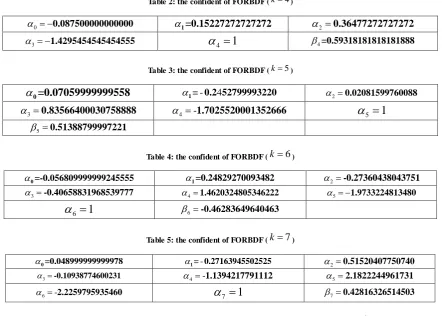
k _{is the confident of}

k

_{order FORBDF, they are given in Table 2 and Table 3}

[image:6.595.85.528.183.499.2]

and Table 4 and Table 5.

Table 2: the confident of FORBDF (k=4)

0

α = −0.087500000000000 α₁=0.15227272727272 α₂=0.36477272727272

3

α = −1.4295454545454555

α =

₄

1

β4=0.59318181818181888

Table 3: the confident of FORBDF (k=5)

α

0=0.07059999999558 α1= 0.2 52799993220- 4 α2=0.02081599760088

3

α =0.83566400030758888 α₄=-1.7025520001352666

α =

₅

1

5

β =0.51388799997221

Table 4: the confident of FORBDF (k=6)

α0=-0.056809999999245555 α1=0.24829270093482 α2=-0.27360438043751

3

α =-0.40658831968539777 α4=1.4620324805346222 α5= −1.9733224813480

6

1

α =

β6=-0.46283649640463

Table 5: the confident of FORBDF (k=7)

α0=0.048999999999978 α1= 0.27163945502525- α2=0.51520407750740

3

α =-0.10938774600231 α₄=-1.1394217791112 α5=2.1822244961731

6

-α = 2.2259795935460

α =

₇

1

β7=0.42816326514503

Here, the approximation of fractional derivative is the same as above. The confident

1 _{( 0,1, 2, , )}

j

w−α j= 2 n+k

determined by the following the coefficients of the Taylor expansion that

1-

α

th power of generating function

v x

( )

, the generating function of 4 to 7 as follows:

( )

_{( )}

(

(

)

)

1

1 2 3 4

4

1

3 2 1 0

/

4

v

x

x

x

x

x

α

α

_α

_α

_α

_α

_β

−

−

₌

₊

₊

₊

₊

( )

_{( )}

(

(

)

)

1

1 2 3 4 5

5

1

4 3 2 1 0

/

5

v

x

x

x

x

x

x

α

α

_α

_α

_α

_α

_α

_β

−

−

₌

₊

₊

₊

₊

₊

( )

_{( )}

(

(

)

)

1

1 2 3 4 5 6

6

1

5 4 3 2 1 0

/

6

v

x

x

x

x

x

x

x

α

α

_α

_α

_α

_α

_α

_α

_β

−

−

₌

₊

₊

₊

₊

₊

₊

( )

_{( )}

(

(

)

)

1

1 2 3 4 5 6 7

7

1

6 5 4 3 3 2 0

/

7

v

x

x

x

x

x

x

x

x

α

α

_α

_α

_α

_α

_α

_α

_α

_β

−

−

₌

₊

₊

₊

₊

₊

₊

₊

The coefficients

(1 )

₍

₎

0,1, 2,

,

j

j

n k

α

ω

−

₌

₊

2

can obtained by Fourier transform is:

(₁ ) 2 (₁ )

( )

0

1

2

i ijk j

v

k

e

e d

i

π

α α j

v

j

π

−

₌

− −

∫

______________________________________________________________________________

Where

k

the number of steps is,

i

is the imaginary unit.

THE APPLICATION OF FRACTIONAL CALCULUS IN VISCOELASTIC MATERIALS

In 1940s, Scott Blair and Gerasimov proposed a model bounded between a Hookean solid (α=o)and a Newtonian fluid

(

α

=

1)

, their relationship is the fractional Newtonian fluid model can be written as

t

u

D

( )

t

α α

σ

（）

=

t

ε

.

Where

σ

and

ε

denote stress and strain, they are the function of time

t

. The coefficient

ut

( 0)

>

is a single material constant (a generalized viscosity:

u

has unites of stress, while

t

has units of time), and exponent

0

1)

α

（

< ≤

α

can be regarded as a second material constant. The experimental results motivated the development of the Scott Blair’s model; on the other hand, Mathematics inspired Gerasimov who was the first to consider an Abel kernel problem for relaxation modulus in Boltzmann’s general theory of viscoelastic.

Bagley and Torvik proved that the molecular theory of Rouse ( for dilute solution of non- cross linked polymer molecules residing in Newtonian solvents) polymer contribution to stress that corresponds to a fractional Newton element whose order of evolution is a half the a=1 / 2_{. They also stated (no proof) that the molecular theory of}

Zimm has a polymer contribution to that corresponds to a fractional Newton element whose order of evolution is two thirds theα=2/3.

Gemant proposed the fractional viscoelastic model at the first, which changed the 1-order derivative to 1/2 derivative of the stress in Maxwell fluid model:

1/ 2

( )

( )

(

u D

t

D t

D t

η

σ

η ε

η ε



+



=

=



1

/



）

where

u

,

η <

0

are material constants. The fractional Maxwell fluid, which is a spring in series with a fractional Newton element, it can be represented as:

1

0 0

( )

( ),

D

t

D

t

t

α α α α

η

t

σ

ηt

ε

σ

t

−

+ +



+



=

=



1



Where

η

（）

>

0

is the viscosity,

t

（）

>

0

is the characteristic relaxation time, the exponent

α

（）

0

< ≤

α

1

is the fractional order which has the same value on stress and strain.

σ

0+_And

ε

0+_{is the value on stress and strain when}

0

t

=

+_{.Then a limited non-uniform initial state of stress is taken into account and Gemant’s model does not possess.}

The fractional Maxwell fluid was first discussed in the manuscript of Caputo and Mainardi as a special case of their material model.

Caputo introduced a fractional Voigt solid 1 ( )

a

t u p Dα t

σ（）= _ + _ε

to model the nearly rate-insensitive dynamic response of Earth's crust over large ranges in frequency when excited by earthquakes. Here

µ

，

p

>

0

and

(0

1)

α

< ≤

α

_{are the material constants. As a mechanical model, this is a spring in parallel with a fractional}

Newton element. A more appropriate representation of solid behavior is the fractional Kelvin model, which is a spring in parallel with a fractional Maxwell element. This material model was introduced by Caputo and Mainardi and has the form:

0 0

( )

1

( ),

p

D

t

p D

t

α α α α

t

ε

µ

ε

σ

ε

t

+ +



+



=



+



=



1







（）

Where

µ

（）

<

0

is the rubbery modulus,

α

µ ρ t

（）（）

/

>

µ

_{is the glassy modulus,}

t

（）

>

0

_{is the characteristic}

considered as a fractional Kelvin model or a fractional standard linear solid model.

CONCLUSION

The fractional order systems are described by fractional differential equations, and the order can be any real number or plurality. The fractional system involve mathematics, physics and cybernetics. In mathematics, it is used in definition of the fractional calculus, analysis and digital implementation. In physics, it is applied in complex system modeling of the fractional calculus. In cybernetics, it is used to expanse the existing control theory to make a better control effect. The fractional calculus is just emerging in the numerical solution, this paper is just the tip of iceberg in numerical solution of fractional differential equation, we just made a preliminary attempt, and there are many questions still need to be further research. Currently, we are working on fractional simulations of the anti circuit and fractional neural networks and so on.

Acknowledgements

This work was supported by National scientific and technological support projects (No.2012BAE09B00), the National Natural Science Foundation of China (No.51274270) and the National Natural Science Foundation of Hebei Province ( No. E2013209215).

REFERENCES

[1]J. Liouville. Journal del Ecole polytechnique Cahier. 1833.14,149–193.

[2]K. T. Vu, R. Gorenflo. Journal of Applied Mathematics and Mechanics.1995. 75(8), 646-648.

[3]S.B. Yester. Journal of Computational Physics.2006. 216, 264-274.

[4]Tatom F B. Fractals. 1995. 3, 17-229.

[5] Mandelbrot B B and Vanness J W . Fractional Noise and Applications.1968.10, 422-437.

[6] Kempfle S.,Schaefer I.,Beyer H. R.. Theory and Applications, Nonlinear Dynamics.2002. 29, 99-127.

[7] X. Z.Lu, F. W. Liu. Numerical Mathematics a Journal of Chinese Universities. 2005. 27(3), 267-273.

[8] B. Bois, K. Mihaly, M. Make. Computer Mathematics with Applications.2008. 55(10), 2212-2226.

[9] R. Lin, F. W. Liu. Journal of Xiamen University (Natural Science). 2004. 43(1), 21-25.

[10]D. Kai, J. F. Neville. Journal of Mathematical Analysis and Applications. 2002. 265,229-248.

[11]S. S. Ray, R. K. Bera. Applied Mathematics and Computation.2006. 174,329-336.

[12]R. L. Bagley and P. J. Torvik. Journal of Rheology. 1983. 27, 201-210.