Investigation of a Boundary Layer Flow near the Inflection Point of a Smooth Curve

(1)

Investigation of a Boundary Layer Flow near the

Inflection Point of a Smooth Curve

J. Venetis

School of Applied Mathematics and Physical Sciences, Section of Mechanics NTUA *Corresponding Author: johnvenetis4@gmail.com

Abstract

In this paper, the author investigates a generic type of the two dimensional incompressible viscous boundary layer flows near the inflection point of a smooth curve. In particular, an approximate evaluation of velocity distribution in an “adjacent” region of the inflection point of this curve is derived. Here, it is a priory assumed that this point is unique. Besides, the flow field is supposed to be steady throughout and Prandtl’s simplified assumptions for two dimensional boundary layer flows are also taken into consideration. Besides, if the cross – section of a structure can be simulated by such a curve one should denote that its inflection point is from technical aspect a very suitable place for emplacing a wind generator compared with the top of a curve, which is a stationary point, because if a wind generator was located on the top of a curve, it could be exhibited in unexpected strong blasts.

K

eywords

Dynamical System, Boundary Layer Flow, Inflection Point, ODE, Stability, Lyapunov’s Criterion

1. Introduction

The approximate analytical solutions of initial or boundary value problems although actually describe simplified cases of the real physical phenomenon, have still the advantage compared with the numerical methods of domain discretization and boundary elements, that help us to study qualitative information, (e.g. asymptotic behavior and stability), for the set of the solutions of the ODE or PDE which illustrates the evolution of the phenomenon we investigate [8,13].

Concurrently, several times one has to study invariant properties in regards to the set of solutions of an ODE under small perturbations and generally to give an answer, although with limited range, to the tracking problem of a dynamical system which can also be a continuum medium, (e.g. a flow field), since an important endeavor has been made in the reform of the classical theory of continuum mechanics in the frame of the Hamiltonian system.

Here, we emphasize, that even a steady flow field can be

several times considered as a dynamical system, because it constitutes an instantaneous image, (or a spot), of an unsteady flow field and indeed every unsteady flow can be encountered as a sequence of instantaneous images of steady flows. Besides, the distinction of a flow field as steady or unsteady many times depends on the type and the position of the circumstantial frame of reference.

Speaking for perturbations of small range, the behaviour of a non – linear dynamical system can be approached by the behaviour of the corresponding linear system. Some of the perturbations are possible to be counted during the “action” of the system and called observed perturbations, whereas some other perturbations cannot be counted and therefore are called non – observed [5]. The signals, (or responses), which are evoked by the perturbations, are competent to transfer information, about the situation of the system, (e.g. mechanical properties of a flow field), and are divided in deterministic, (e.g. laminar flow field) and stochastic (e.g. turbulent flow field).

However, the latter of these systems are called in general: “Random Fluctuation Systems”, just because the input of energy and matter as well, occurs on an irregular time schedule [1,6].

Therefore, if a flow field is considered as a dynamical system, one may derive qualitative information about its most important characteristics such us controllability, observation ability, eigenvalues and mainly stability, by the use of approximate analytical expressions for some significant quantities such as velocity.

Next, speaking for boundary layer flows, we can report from the literature that the first exact solution to Prandtl’s equations, which are the governing equations for such flow patterns, was derived by Blasius via a combination of differential and dimensional analysis of the flow field [6]. The main assumption of this method is that the dimensionless parameter

V

x

/

V

∞ depends on the tangential

(2)

shape of the velocity profile [15]. This method, which is also known as Momentum Integral Method, changes the two Prandtl’s PDEs into a single differential equation which is applicable only when the pressure gradient term is zero. Moreover, in regards to the existence and properties of analytical solutions to unsteady Prandtl’s equations a remarkable progress was made, as it can be seen in Refs. [12, 16,17].

On the other hand, an alternative exact closed – from solution to Prandtl’s equations, has been proposed by Venetis et al without dimensional arguments and functional notations with respect to any characteristic sizes of the flow [14].

In this work, we will also deal with the two dimensional incompressible viscous boundary layer flow past a smooth curve, but on the contrary with the above aforementioned approaches, we will focus our study only on an “adjacent” region of the inflection point of this curve without trying to derive an expression of the governing velocity component along the boundary layer.

2. Estimation of Transverse Velocity

Distribution Past the Inflection Point

of the Curve

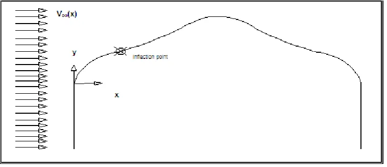
In the general case of a flow field around a mounted obstacle whose cross - section formulates a smooth curve, one may select a motionless coordinate system located at the leading edge of the mounted obstacle which is considered as a rigid body instead of a moving coordinate system which is in accordance with Lagrangian formalism.

Evidently, this curve can be considered without violating the generality, as the graph of a single – valued function in the form

y

=

y

(

x

)

Here, one may distinguish three cases regarding this function.

We initiate our investigation, supposing that the function

)

(

x

y

[image:2.595.118.497.331.494.2]

y

=

is strictly concave before the inflection point of the curve as it can be seen in Fig.2.

Figure 1. Motionless Cartesian Coordinate System (Eulerian Formalism)

[image:2.595.114.495.461.700.2]

(3)

The component of the flow velocity which is parallel to axis xx΄ is described by a continuous function

)

(

y

V

x

=

x [11]. Therefore, it can be defined as a

continuous composed function in the form:

y

V

x

V

x

(

)

=

x

°

Obviously, by assuming that this function is twice differentiable, we can use the chain rule which is formulated here in Leibniz representation

dx

dy

y

V

x

V

x x

_⋅

∂

=

∂

(1)

Besides, Prandtl’s equation of momentum conservation holds for the axis xx΄[6]:

dx

dP

y

V

y

V

x

V

x x

y x

x



=

∂

_∂

−

⋅











∂

+

∂

µ

ρ

1

2 2 (2)

where:

P

=

P(x)

, denotes the sum of barometric and manometric pressure, and it can be specified via the external local velocity

V

_e, which occurs on Ekman’s equations for the atmospheric boundary layer , but mostly is assumed to be motivated by a potential flow field [6].

On the other hand, as it is known from Vector Calculus the following identity holds [2]

(

)

( )

(

)

(

)

2 2 2 2 2 2 2 2 2 2

2

1

2

1 y

V

x

V

x

V

x

V

y

x

V

x

V

x

V

y

V

x

V

div

grad

V

grad

V

grad

V

y x y x y x y x y x

∂

+

∂

+

























∂

+

∂













∂

+

∂

−













+

∂

+

∂

⋅

=

∇

+

−

=

⋅



(3)

The identity above can arise from a combination of the following two elementary identities of Vector Calculus [2]: a)

grad

(

div

V



)

=

grad

×

(

grad

×

V



)

+

∇

2

V



b)

grad

V



2

=

2 (

V



⋅

grad

)

⋅

V



+

2 V



×

(

grad

×

V



)

Besides, the assumptions of Prandtl’s formalism are the following [6]: 2 2 2 2

;

y

V

x

V

y

V

x

V

x x x x

x y

_∂

∂

<<

∂

<<

∂

<<

Thus, eq. (2) , can be modified as follows

⇒

∂

+

⋅

−

=

























∂

2 2

1 y

V

dx

dP

x

V

x x

x

_µ

µ

ρ

2 2

1 dy

V

d

dx

dP

dx

dV

V

x x

x



=

−

_ρ

⋅

+

µ











₍₄₎

Here, we have taken into account that

V

x

=

V

x

(

y

)

Hence, we have arrived to a linear ODE. Here, we remark that Prandtl’s formalism for a motionless Cartesian frame of reference, holds only for planar surfaces or curves with faint curvature, therefore we shall focus our study on an “adjacent” region on the graph

y

=

y

(

x

)

, around the inflection point, (which is the mapping of a

ε

−

neighbourhood at the domain of definition of the function

y

=

y

(

x

)

with centre point the rate x0). Besides, for every point of the cross – section of the curve, represented in the form:

y

=

y

(

x

)

, it is valid that:

V

_x

=

0

(no– slip boundary condition), so if we neglect the term in the left member of eq. (4), taking into account Taylor’s representation for the multi – valued function:

V

_x

(

x

,

y

)

in accordance with Prandtl’s aforementioned assumptions, we can obtain:

dx

dP

y

x

V

x y

y

=

⋅

∂

=

_µ

1 )

(

) ( 2 2 (5)

Also, at the windward side of the curve there exist favourable pressure gradients i.e.

≤

0 dx

dP

_{, so we deduce}

0 )

(

2 2

≤

∂

y

V

x (6)

The last inequality, informs us that the function of velocity distribution

V

_x

(

y

)

over the curve, is concave, if we stipple the graph:

V

_x

=

V

_x

(

y

)

In fact the pressure gradient force tends to cause the fluid to accelerate in the direction of the pressure gradient.

We can pinpoint here, that the existence of the pressure gradient which actually constitutes a directional derivative, does not imply necessarily and sufficiently the continuity of the function

P(x)

. Hence, the total derivative of velocity which is equal to the convective acceleration

(

V



⋅

∇

)

⋅

V



can be seen as the directional derivative of this quantity, in the direction of the pressure gradient. Currently, it is also known that the magnitude of this force is proportional to the steepness of the pressure gradient. On the inflection point of the curve with coordinates (x0, y0), the two following

conditions are valid:

1. - From Fluid Dynamics viewpoint:

(4)

The above relationship arises from the fact, that the inflection point of the curve is many times a critical point for an external flow field, where one starts to observe adverse pressure gradients, i.e.

≥

0 dx

dP

_{, which are the main reason}

for boundary layer separation) [2,6,9]. Here, we should denote that the exact position of the separation point is determined via the solution of the equation:

0 )

(

0

=

= y x

dy

y

dV

where y is now the normal distance from the solid surface. The rate of this distance can be expressed with respect to the coordinates of the frame O x,y,z if we know the distance of this point from the origin, as well as the rate of the derivative

dx

dy

_{at this point.}

2.- From Single - Valued Calculus aspect:

0 )

(

2 0 0 0 2

=

dx

x

y

d

(8)

Thus from eq. (5), taking into account eq. (7), we can obtain the following relationship:

⇒

=

∂

(

)

₀

2 0 0 2

y

V

x

⇒

+

=

∂

1 0

0

)

₍

₎

(

_f

_x

_c

y

V

x 2 2 0 1 0 1

0

)

(

)

(

)

(

y

c

y

f

x

y

f

x

c

V

x

=

⋅

+

⋅

+

(9)

If we concentrate on an “adjacent” region of the inflection point (x0, y0) eq. (9) can be written out in the form:

2 2

1

(

)

(

)

(

y

c

y

f

x

y

f

x

c

V

_x

=

⋅

+

⋅

+

(10)

Obviously, because of the nature of the original problem that we investigate, the domain of definition of the function

)

(

y

V

x

=

x is bounded. Hence, by making the assumption that the functions

f

₁

,

f

₂ are continuous, it implies that

f

₁

(

x

)

<

∞

∧

f

₂

(

x

)

<

∞

.

In the sequel, an application of the no – slip boundary condition yields

0 )

,

(

x

0

y

0

=

V

x

⇔

c

1

⋅

y

0

+

f

1

(

x

0

)

⋅

y

0

+

f

2

(

x

)

+

c

2

=

0

(11)

Next, if we differentiate the above equation with respect to variable x, we obtain

0 )

(

)

(

)

(

2 1 1

1

⋅

+

⋅

+

⋅

+

_dx

=

x

df

dx

dy

x

f

y

dx

x

df

dx

dy

c

(12) In the range of validity of eq.(11), the function

y

(

x

)

is called linear approximation or linearization of the function

whose graph describes the cross – section of the obstacle, in the “adjacent” region of the inflection point (x0, y0).

Thus, we deduce:

(

₀

)

0

)

(

)

(

)

(

₀

x

dx

dy

x

y

x

L

x

y

=

_x

=

+

⋅

−

(13)

where

lim

(

)

0

(

)

0

x

L

x

y

_x x x

−

→

=

0

Concurrently, by integrating twice eq. (8) one obtains













₊

⋅

=

+

⋅

=

a

b

x

a

b

x

a

y

₀ ₀ ₀ (14)

where α,b

∈

R

*

Thus, eq. (11), in the neighbourhood of inflection point, can be represented as follows:

(

+

)

+ ⋅ + = ⇒

⋅ +

⋅ ( ) ( ) ( ) 0

0 2 1 1 dx x df a x f b x a dx x df a c

⇒

=

⋅

+











 +

⋅

+

(

)

(

)

1

2

(

)

0

1 1

1

df

_dx

x

_a

b

f

x

_a

df

_dx

x

c

dxx df b x a a b x c a b x x f dxx

df( ) ₍ ₎ 1 1 1 2( )

1 1 _⋅ + ⋅ − + − = + ⋅ + (15) This ODE above, belongs to the general form

)

(

)

(

)

(

)

(

_f

_x

_h

_x

dx

x

df

₊

_⋅

_φ

₌

_{, (with the assumption that:}

)

(

x

φ

and

h

(

x

)

are continuous functions), which is generally integrable. Here, dx x df b x a a b x c x h a b x

x) 1 ; ( ) 1 ( )

( 1 _⋅ 2

      + ⋅ − + − = + = φ

The general solution of eq. (15) is:

(

x dx

)

(

k

(

h x EXP

(

xdx

)

dx

)

k R x f ∈ ∀ ⋅ + ⋅ =

∫

( ) ( ) ( ) -EXP ) ( 1 φ φ (16) where:

(

)

_x

_a

b

a

b

x

d

a

b

x

dx

x



=

−

+









 +

+

−

=

∫

(

)

1 ln

-

φ

So it implies that

(

)

a b x a b x dx x + =      ₋ ₊ =

∫

( ) EXP ln 1

(5)

Besides, it is also valid             ⋅             + + + − =             ⋅       + ⋅ + + − = dx x df a b x a a b x c dx x df b x a a b x c x h ) ( 1 1 ) ( 1 ) ( 2 1 2 1

Then we can obtain:

(

)

(

)

dx a b x dx x df a b x a a b x c dx dx x x h + ⋅             ⋅             + + + − = ⋅

∫

) ( 1 1 ) ( EXP ) ( 2 1 φ ) ( 1 ) ( 1 2 3 1 2

1 _a df_dxx dx c x c _a f x

c  =− ⋅ + + ⋅

     + − =

_∫

∫

Hence, with eq. (16) in hand in accordance with the above date, we deduce













₋

_⋅

₊

_⋅

⋅

+

=

1

1 (

)

(

1 3 2

1

k

c

x

c

_a

f

x

a

b

x

f

(17)

Thus, for the “adjacent” region of the inflection point, eq.

(10), yields

⇒

+

⋅

+

⋅

=

₁ ₁

(

)

₂

(

)

₂

)

(

y

c

y

f

x

y

f

x

c

V

x

⇔

+

⋅

























₋

_⋅

₊

_⋅

⋅

+

⋅

=

2 2 2 3 1 1

)

(

)

(

1

1 )

(

c

x

f

y

x

f

a

c

x

c

k

a

b

x

y

c

y

V

_x 3 2 1 2 2 2 3 1 1

,

)

(

)

(

1 )

(

c

x

f

x

f

a

c

x

c

k

a

b

x

y

c

y

V

x

∀

+













₋

_⋅

₊

_⋅

⋅

+

⋅

=

(18) Next, eliminating of the fractions whose denominators have exponents “+ 2”, we can obtain the following rational form:

(

₁ ₃

)

₂ ₂

1

(

)

(

k

c

x

c

f

x

c

a

b

x

y

c

y

V

x

⋅

−

⋅

+

⋅

=

(19)

Since in the neighbourhood of the inflection point of the

curve it is valid that











 +

⋅

=

a

b

x

a

y

we deduce

(

1 3

)

2 2

1

(

)

(

y

c

y

a

k

c

x

c

f

x

c

V

x

=

⋅

+

⋅

−

⋅

+

(20)

Then, if we consider that the independent value

x

belongs

to the set: _

     ₊ ∪       ₋ a b x x x a b

x0 , 0 0, 0 in accordance

with the assumption:

y

V

x

V

x x

∂

<<

∂

we can arrive to the following approximate rational representation:

3 2 1

1 )

(

C

y

C

y

C

y

V

_x

=

⋅

+

⋅

+

(21)

where

C

₁,

C

₂,

C

₃ are arbitrary real constants which depend only on the occasional boundary conditions.

We observe that this expression above, is a sum of a first degree polynomial function and a homographic function 1. According to the nature of the original problem we study, the maximum value of velocity inside boundary layer is the 99% of the external local velocity

V

_e along the boundary layer. This velocity is generally different from the free stream velocity which concerns planar surfaces but indeed can arise from a frictionless flow field outside the boundary layer. It depends on the transposition of the leading edge of the obstacle. Apparently, the behavior of these functions in the “adjacent” region of the inflection point (x0, y0), approaches

the behaviour of the corresponding first degree polynomial function Q(x)=C₁⋅y+C₃

Obviously, this function has not asymptotic behavior compared to the family of the functions of velocity distribution around a mounted obstacle. Moreover, we primarily assumed that the function

V

_x

(

y

)

is concave in the windward side of the curve.

Hence, from Single – Valued Calculus [6] the following inequality holds:

(

₀

)

0 0 0

)

(

)

(

)

(

y

dy

y

dV

y

V

y

V

x x

x

≤

+

⋅

−

(22)

So we can conclude

0 % 99 0 % 99 0

0

)

(

)

(

)

(

y

V

y

V

dy

y

dV

e V e V

x

−

≥

(23)

1_{Every homographic function:}

δ γ β α σ + + = y y y)

( can be written out in the form:

µ λ γ δ γ αδ βγ γ α σ + + = + − + = y k y

y) 2 (

(6)

where:

y

₉₉_%

y

₀ e

V

−

is the thickness of boundary layer at the position (x0,y0 ).

Hence, we deduce that the velocity distribution, in the region we study, will approach the external local velocity:

V

_e, (which is actually its maximum value), with a greater rate of change:

y

V

x

∆

(

)

_{, than its corresponding evident rational}

approximation. Thus, we can conclude that the inflection point of the curve is from the aspect of fluid dynamics as well, the most suitable part of a curved mounted obstacle, for emplacing a wind generator.

We can try to investigate the stability of this solution, by using Lyapunov’s definition of the stability of an ODE.

The general form of this solution is: 3 2

1

1 )

(

C

y

C

y

C

y

V

x

=

⋅

+

⋅

+

Αt the inflection point we have:

V

_x

(

y

₀

)

=

0

(no - slip condition)

Let us consider the following difference:

3 2

1

3 2

1 0

1

0 )

(

)

(

C

y

C

y

C

y

C

y

C

y

V

y

V

x x

+

⋅

+

⋅

=

−

⋅

−

⋅

−

=

−

For every rate of the evident solution the following mathematical statement holds:

If

1

3

(

)

0 2 0

1

⋅

y

+

C

⋅

_y

+

C

<

δ

ε

C

⇒

ε

<

+

⋅

+

⋅

₂ ₃

1

y

C

1 C

_y

C

There, we can consider that:

(

₉₉_% ₀

)

(

ε

=

ε

−

y

_V_e

−

y

δ

_,

where

(

y

₉₉_%

y

₀

)

e

V

−

is the thickness of boundary layer

over the inflection point (x0 ,y0).

Obviously for this point, (in particular at the “adjacent” region of it), the following inequality holds

(

₉₉_% ₀

)

0

<<

−

>

−

=

∆

_y

_V_e

_y

(24)

So we infer:

⇒

−

<

+

⋅

+

⋅

1

₃

(

₉₉_% ₀

)

0 2 0

1

y

C

y

C

y

C

e V

ε

≥

−

+

⋅

+

⋅

>

)

(

1

0 %

99

3 0

2 0

1

y

C

y

C

y

C

e V

ε

(

)

3 2

1

3 0

2 0

1

0 %

99 3

0 2 0

1

1 )

(

1 C

y

C

y

C

y

C

y

C

y

C

y

C

y

C

e V

+

⋅

+

⋅

>

+

⋅

+

∆

+

⋅

>

−

+

⋅

+

⋅

Hence we can establish that the solution is stable at the “adjacent” region of the inflection point.

Besides, we can also find that:

∞

+

=

+

⋅

+

⋅

=

−

∞ + →

3 2

1 0

1 lim

)

(

)

(

lim

C

y

C

y

C

y

V

y

V

y

x x

y

(25)

Hence, the solution is not asymptotically stable at the inflection point.

Second case

(7)

Figure 3. Strictly Convex Curve Third case

[image:7.595.110.501.77.267.2]

However, in case that the curve has no inflection point and obviously Prantdl’s formalism is not valid, we can use transversely the following diagram from Euro - Code 2 [Fig.4] which has been gathered by experimental approach using building models in wind tunnels:

Figure 4. Inflection Point at the Top of the Curve

3. Discussion

As we have already denoted, an analytical solution, though in an approximate form, is very helpful to sypply qualitative information such us stability for the set of the solutions of an ODE. In our case, it can serve as a useful strict test for an explicit expression of the governing velocity component.

Nevertheless, such qualitative results linking the governing velocity component of a boundary layer flow and its critical properties, could be useful for those desiring to identify beforehand the ranges of velocity for a flow field past a smooth curve where inflection points are likely to be found.

Besides, the contribution of the curvature of a mounted obstacle which is inserted into a flow field concerning Tollmien - Schlichting’s instability [2,7,9], is not very significant. Apart from these aforementioned instabilities, there are some other ones due to the centrifugal forces which are created exactly by the curvature of the mounted obstacle. The general pattern of these instabilities is a sequence of eddies, which are called Görtler eddies. The Görtler eddies appearing mainly on a concave wall,

[image:7.595.112.502.349.566.2]

(8)

following relationship becomes greater than 1.2. , i.e.

2 .

1 Re

*

>

=

R

G

δ

Next, speaking for the impact of the roughness of the surface, it is also known that from Fluid Dynamics viewpoint that a surface is called “smooth”, when its roughness is less than the thickness of viscous sub layer which is at least the 1% of the thickness of the self -preserving turbulent boundary layer. However the convergence of stream lines in a three dimensional flow field around a mounted obstacle with random shape, has several times significant changes from the corresponding two dimensional flow field, hence it could be studied in the Euclidean space, by designing an isometric projection of the obstacle and following Computational Fluid Dynamics methods, provided of course that it is known either the geometry of the obstacle or velocity distribution on the exterior bound of it which necessarily must be assumed to constitute a piece – wise smooth, simply closed and not self – intersected mathematical surface, which verifies Jordan Criterion of rectilinerability.

4. Conclusions

In this paper, the author attempted to derive an approximate analytical evaluation of velocity distribution in an “adjacent” region of the inflection point of a curve, over which a boundary layer incompressible flow takes place.

Here we should emphasize, that the objective of this work is not the presentation of a closed – form expression of the governing velocity component along the boundary layer, but the obtainment of an approximate algebraic expression for velocity field for an “adjacent” region of the inflection point of this curve.

To this end, Prandtl’s simplified assumptions for two dimensional boundary layer flows have been also taken into account.

In addition, we also deduced that the inflection point of the curve is from fluid dynamics viewpoint, the most suitable part of a curved mounted obstacle, for emplacing a wind generator.

REFERENCES

[1] Kacmal J.C., Finnigan J.J. Atmospheric Boundary Layer Flow Oxford Unvercity Press, 1994

[2] Hilbebrandt F. Advanced Calculus for Applications, second edition Prentice – Hall New Jersey, 1976

[3] Ladyzhenskaya. O.A. The mathematical theory of viscous incompessible flow Second English edition. Translated from the Russian by R.A. Silverman and J. Chu. Gordon and Breach Science Publishers New York 1969 (reprint 1975) [4] Lions P.L. Mathematical topics in fluid mechanics Vol. 1

Incompressible models Oxford Lecture Series in Mathematics and its Applications 3 Oxford University press 1996

[5] Paraskevopoulos P.N. Introduction to Automatic Control Systems, Marcel Dekker 1999

[6] Schlichting H. Boundary Layer Theory, 7th Edition, Mc Graw Hill, New York, 1979

[7] Stull R.B. An Introduction to Boundary Layer Meteorology Kluwer Academic Publ. 1989

[8] Tyn Myint. Partial Differential Equations of Mathematical Physics Elsevier Scientific Publ. Company New York 1976 [9] Yeang Ken. The skyscraper bio - climatically considered Ν.Υ.

Academy Editions, 1996

[10] Falkner V.M., Scan B., Solutions of the boundary-layer equation, Philosophical Magazine Series 7, Volume 12, Issue 80, pages, 865-896, 1931

[11] Howarth L., On the Solution of the Laminar Boundary Layer Equations, Proceedings of the Royal Society of London. Series A, Mathematical and Physical Sciences, Vol. 164, No. 919 (Feb. 18, 1938), pp. 547-579

[12] Oleinik, O., On the mathematical theory of boundary layer for unsteady flow of incompressible fluid, Journal of Appl. Math. Mech. 30, 1966, pp. 951–974.

[13] Rassias J.M. Counter Examples in Differential Equations and Related Topics World Scientific, Singapore 1994

[14] Venetis J., Sideridis E., On a Closed – Form Solution of Prandtl's System of Equations International journal of fluid mechanics research Vol. 40 Issue 2 pages 106-114, 2013 [15] Von Karman T., Millikan C., On the theory of laminar

boundary layers involving separation, 1934 aerade.cranfield.ac.uk

[16] Weinan E., Enquist B. Blow up of solutions of the unsteady Prandtl's equation Comm. Pure Appl. Math., 50 (1998), pp. 1287–1293