PARIS RESEARCH LABORATORY
d i g i t a l
April 1994
J ´er ˆome Barraquand
Didier Martineau
Numerical Valuation
of High Dimensional Multivariate
American Securities
J ´er ˆome Barraquand
Didier Martineau
The authors can be contacted at the following addresses:
Jerome Barraquand
Digital Equipment Corporation Paris Research Laboratory 85 Avenue Victor Hugo
92500 Rueil-Malmaison, France
Didier Martineau
Digital Equipment Corporation Paris Research Laboratory 85 Avenue Victor Hugo
92500 Rueil-Malmaison, France
c
Digital Equipment Corporation 1994
We consider the problem of pricing an American contingent claim whose payoff depends on several sources of uncertainty. Using classical assumptions from the Arbitrage Pricing Theory, the theoretical price can be computed as the maximum over all possible early exercise strategies of the discounted expected cash flows under the modified risk-neutral information process.
Several efficient numerical techniques exist for pricing American securities depending on one or few (up to 3) risk sources. They are either lattice-based techniques or finite difference approximations of the Black-Scholes diffusion equation. However, these methods cannot be used for high-dimensional problems, since their memory requirement is exponential in the number of risk sources.
2 Relation to other work
43 Arbitrage pricing theory
53.1 Diffusion model of information process : : : : : : : : : : : : : : : : : 5
3.2 European securities : : : : : : : : : : : : : : : : : : : : : : : : : : : : 5
3.3 Arbitrage pricing : : : : : : : : : : : : : : : : : : : : : : : : : : : : : : 6
3.4 American securities : : : : : : : : : : : : : : : : : : : : : : : : : : : : 7
3.5 European and American options : : : : : : : : : : : : : : : : : : : : : 8 3.5.1 European options : : : : : : : : : : : : : : : : : : : : : : : : : : 8 3.5.2 American options : : : : : : : : : : : : : : : : : : : : : : : : : : 10
4 Numerical methods for American security pricing
114.1 Stochastic dynamic programming : : : : : : : : : : : : : : : : : : : : 11
4.2 Finite differences and the Cox-Ross-Rubinstein approach : : : : : : : 12
5 State aggregation
145.1 State aggregation price : : : : : : : : : : : : : : : : : : : : : : : : : : 14
5.2 Markovian approximation : : : : : : : : : : : : : : : : : : : : : : : : : 15
5.3 Recursive state aggregation : : : : : : : : : : : : : : : : : : : : : : : 16
5.4 Stratified state aggregation (SSA) : : : : : : : : : : : : : : : : : : : : 17
6 Monte Carlo estimation of American price
196.1 Generation of sample paths : : : : : : : : : : : : : : : : : : : : : : : 19
6.2 Conditional probabilities and payoff expectations : : : : : : : : : : : : 19
6.3 Backward integration algorithm : : : : : : : : : : : : : : : : : : : : : : 20
7 Quadratic resampling
207.1 Quadratic resampling for multidimensional Monte Carlo integration : : 20
7.2 Quadratic resampling in spacetime : : : : : : : : : : : : : : : : : : : 22
8 Experimental results
228.1 A test case : : : : : : : : : : : : : : : : : : : : : : : : : : : : : : : : : 22
8.2 One underlying asset : : : : : : : : : : : : : : : : : : : : : : : : : : : 24
8.3 Two underlying assets : : : : : : : : : : : : : : : : : : : : : : : : : : : 24
8.4 Three underlying assets : : : : : : : : : : : : : : : : : : : : : : : : : : 29
8.5 Ten underlying assets : : : : : : : : : : : : : : : : : : : : : : : : : : : 29
8.6 Efficiency of extended quadratic resampling : : : : : : : : : : : : : : 32
8.7 Experimental time complexity : : : : : : : : : : : : : : : : : : : : : : : 32
8.8 Parallel implementation : : : : : : : : : : : : : : : : : : : : : : : : : : 33
1
Introduction
Since the seminal work of Black and Scholes (1973) and Merton (1973) in the early 1970s, the arbitrage principle underlying option valuation theory has been extended to a broad range of other financial instruments (see e.g. Ross (1976), Cox and Rubinstein (1985)). Indeed, any security whose returns are contractually related to the returns on some other security or group of securities can theoretically be valuated using the same arbitrage principle. In some cases, explicit closed form analytical formulas for the computation of the arbitrage price can be derived from this theory. In particular, the original paper of Black and Scholes (1973) provides a closed form solution for a European option on a single common stock. Unfortunately, few other cases can be solved analytically, and computing the arbitrage price often requires numerical simulations. Following an idea initially presented in an early edition of Sharpe (1985), Cox et al. (1979) developed a discrete model for the valuation of an American option on a single stock that can be easily computed numerically. However, the effective implementation of the arbitrage principle is not always such an easy task, and may sometimes become intractable. Tractable algorithms have been developed recently for pricing European contingent claims with many underlying assets (see e.g. Barraquand (1993)). However, these algorithms cannot be used for pricing American contingent claims.
There are several reasons motivating the development of efficient methods for multidimensional contingent claim pricing. In particular, applications exist in the pricing of Over The Counter (OTC) warrants, path dependent instruments (Barraquand and Pudet (1994)), multidimensional interest rate term structure contingent claims (Heath et al. (1992)) such as mortgage-backed securities, and life insurance policies (Fabozzi and Pollack (1987)), futures contracts with quality delivery options (Cheng (1987); Boyle (1989)). Also, pricing models taking into account the stochastic nature of volatility (Wiggins (1987); Dothan (1987); Hull and White (1988)) require multidimensional modeling. Other applications exist in assets and liabilities management, and in corporate capital budgeting (see e.g. Mason and Merton (1985); Coppeland (1989); Brealey and Myers (1991)). Finally, applications exist in property/liability insurance (Merton (1977); Smith (1979); Kraus and Ross (1982); Doherty and Garven (1986); Cummins (1988); Shimko (1992)). The tremendous development of financial engineering during the past decade can be expected to continue, and new types of securities requiring multidimensional modeling are likely to appear at a sustained pace in the future.
call American instruments all financial assets belonging to this second class.
Following the general theory of arbitrage pricing, the theoretical price of a European contingent claim is the discounted expected value of its future cash flows under the so-called “risk-neutral” probability distribution of the underlying economic factors (Harrison and Kreps (1979); Harrison and Pliska (1981); Duffie (1988); Karatzas and Shreve (1988)). Mathematically, computing the arbitrage price reduces to computing an integral (sum) over the space of the underlying economic factors. When the dimension of the space of the underlying economic factors is small, standard techniques for numerical integration can be used. In some cases, the integral can even be computed analytically (e.g. Black-Scholes formula). However, the computational complexity of evaluating the integral is clearly exponential in the dimension of the space. Efficient numerical techniques for pricing high-dimensional European claims are presented in Barraquand (1993).
The price of an American claim is the maximum over all possible cash flow monitoring strate-gies of the associated present values of cash flows. For example, the price of an American option is the maximum over all possible early exercise strategies of the corresponding present values. Since the space of cash flow monitoring strategies is generally huge, direct maximiza-tion of the present value is rarely practical (see Bossaerts (1989) for a discussion). However, when the underlying economy is modeled as a Markov process, one can use the Bellman principle of dynamic programming (Bellman (1957)) to compute the optimal monitoring strat-egy. American options are typically priced using a discrete approximation of the dynamic programming principle. This is the case in particular of the CRR model (Cox et al. (1979)) for American stock option pricing. This approach becomes however impractical when the underlying economic space has many dimensions, since the dynamic programming algorithm requires a memory space exponential in the number of dimensions. This fact is known as the “curse of dimensionality” problem for dynamic programming.
In this paper, we present a particular state space partitioning technique that attempts to circum-vent the curse of dimensionality problem for American security pricing. More precisely, we partition the space of underlying assets (the state space) into a tractable number of cells, and we compute an approximate early exercise strategy that is constant over those cells. The hope is that, if the partition is appropriately chosen, the approximate strategy will be close to the actual optimal strategy. Such a partitioning technique is classically called a state aggregation technique.
the technique Stratified State Aggregation along the Payoff (SSAP).
After quantization of the payoff, the SSAP method can be combined with Monte Carlo sim-ulation techniques in order to compute the set of conditional probabilities corresponding to changes in the payoff value over time. Using these conditional probabilities, an approximation of the American price can then be computed backwards in time using techniques reminiscent from the classical CRR integration method.
We implemented the SSAP method on American option pricing problems in dimensions ranging from 1 to 400. On all problems for which we could compare the SSAP method with known optimal solutions, the SSAP price was indistinguishable from the optimal theoretical price. In particular, in dimensions 1, 2, and 3, both put and call prices of options on the maximum of the underlying assets were computed accurately by the SSAP method. Also, the SSAP price of an American call on the maximum of n assets paying no dividends was indistinguishable from the European price for n ranging from 1 to 400, in accordance with a well known theoretical result1. In other cases, no other method exists to compare to our results. However, the SSAP price seems to constitute an accurate approximation of the American price in arbitrarily high dimensions.
To the best of our knowledge, the SSAP method is the first capable of computing American prices and exercise strategies in high dimensional cases.
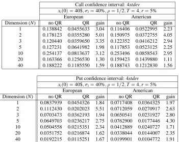
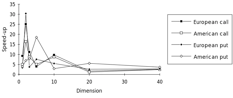
In order to speed-up the Monte Carlo simulation of conditional probabilities, we developed an original variance reduction technique called Quadratic Resampling. Quadratic Resampling was originally presented in Barraquand (1993) for European security pricing. In this paper, we present an extension of the original QR method that applies to both European and American asset pricing problems. Quadratic Resampling consists in correcting the samples obtained through classical Monte Carlo simulation in such a way that the expected value of any polyno-mial of degree two or less in the space variables is computed exactly. Our experiments show that QR is very efficient for American pricing problems in up to 10 dimensions. The average speedup obtained through QR ranges from 5 to 35, with an average of about 10. In higher dimensions (11 and higher), the speedup is only of 2 to 3 in average, and slowly decreases with the dimension.
We implemented a parallel version of the SSAP method on a network of workstations equipped with a high-bandwidth interconnect (called a workstation farm). We observed a speedup linear in the number of workstations in the network. Both measured and simulated parallelization experiments are reported in this paper.
This paper is organized as follows. In Section 2, we relate our contribution to previous work in American security pricing, multidimensional asset pricing, and Monte Carlo valuation. In Section 3, we recall the usual assumptions on the stochastic processes governing the evolution of securities prices, and the main results of the Arbitrage Pricing Theory. In Section 4, we 1Indeed, since the discounted prices of assets paying no dividends are martingales under the risk neutral measure,
briefly review the current numerical methods used for American security pricing. In Section 5, we present the method of Stratified State Aggregation. In Section 6, we show how SSA prices can be computed through Monte Carlo simulation. In Section 7, we present the method of Quadratic Resampling. In Section 8, we present numerical experiments illustrating the efficiency of the SSAP method.
2
Relation to other work
The theoretical analysis of optimal stopping times for early exercise of American options dates back to the work of McKean (1965). This theory has then been further developed by several authors (Merton (1973); Harrison and Kreps (1979); Bensoussan (1984); Karatzas (1988); Jaillet et al. (1988)). Myneni (1992) surveys the theory of American option pricing.
The most widely used valuation technique for American options with one underlying asset is the binomial lattice approach of Cox et al. (1979). Cox and Rubinstein (1985) outline the principle of the multidimensional extension. Other numerical valuation techniques are presented in Geske and Johnson (1984), Barone-Adesi and Whaley (1987), Barone-Adesi and Elliott (1991).
The valuation of options depending of several underlying assets has been extensively studied. Brennan and Schwartz (1979) addresses the problem of pricing options under two sources of risk by direct finite-difference approximation of the generalized Black-Scholes equation. In this example the two sources of risk are the short term and the long term interest rates. The approach is clearly limited to a few assets, since the memory space requirements and the computation time are both exponential in the number of underlying assets. Boyle et al. (1989) developed a multinomial lattice method for pricing multidimensional options, in the spirit of the approach outlined in Cox and Rubinstein (1985). According to the authors, the computation becomes very burdensome for more than two assets. In fact, the multinomial lattice approach can be viewed as a finite-difference approximation of the generalized Black-Scholes equation using an explicit Euler scheme and an appropriate change of variables (Brennan and Schwartz (1978)).
Stulz (1982) presents an analytical solution to the problem of pricing a European option on the maximum or minimum of two underlying assets. The analytical solution is generalized in Johnson (1987) to the case of an arbitrary number of assets, taking as given the cumulative multivariate normal distribution function. Boyle (1989) and Boyle and Tse (1990) developed an approximate method for the same problem. Although the problem is solved analytically in Johnson (1987), the approximate method does not require preliminary computation of the cumulative multivariate normal distribution function. To the best of our knowledge, no closed form solutions have ever been obtained for American pricing problems.
The application of the Monte Carlo method to option pricing was first presented in Boyle (1977), in the context of claims contingent to a single underlying asset. It has then been used by several authors for the valuation of path dependent contingent claims. In particular, the method has been used for pricing mortgage-backed securities (see Schwartz and Torous (1989), Hutchinson and Zenios (1991)). Barraquand (1993) presents the method of Quadratic Resampling for Monte Carlo valuation of European securities with many underlying assets. The Quadratic Resampling method presented in this paper is an extension of this earlier work to the American pricing problem.
3
Arbitrage pricing theory
The arbitrage pricing theory is described in many textbooks. We refer the reader to Duffie (1992) for a comprehensive and rigorous presentation. In the following, we briefly present through intuitive arguments the main results of the theory. These developments do not constitute mathematical proofs, and are only aimed at illustrating the main concepts underlying the computational approaches to arbitrage pricing.
3.1 Diffusion model of information process
We model the economy as a finite-dimensional vector of real-valued state variables X(t) = (x1(t);:::;xn(t)), called factors, representing all the information available to investors at time t. Since X(t)represents all information available to agents at time t, in a frictionless market, prices of securities must be deterministic functions of time and X(t). It is said that securities are contingent claims on the state variable X(t).
For the sake of simplicity, we will assume that the information process X(t) is a diffusion process. However, our results on security valuation described in the next sections apply to more general types of stochastic processes. If X(t)is a diffusion process, it is a solution of a stochastic differential equation of the type (It ˆo and McKean (1965)):
dX =A(X(t);t)dt+B(X(t);t)dW (3.1)
The vector A is called the drift of process X. A is the derivative of the expected value of X.
The matrixΓ=BB
Tis the derivative of the covariance of X. The vector W
=(w1;:::;wn)is a n-dimensional standard Brownian motion.
Often, the variables xiare prices of securities available on the market, and are therefore strictly positive processes. The expected increments and covariance of increments are then expressed in relative values:
8i2[1;n];
dxi xi
=x
i(x1;:::;xn;t)dt+
n
X
j=1
vij(x1;:::;xn;t)dwj
with
x
The matrix V =(vij) (i;j)2[1;n
]2is called volatility matrix, and the covariance of relative returns is the matrixK=(kij)
(i;j)2[1;n ]2:
K=VV
T
3.2 European securities
A security is called European security iff future cash flows cannot be influenced by decisions from the holder taken after the purchase date (besides of course selling back the security). Then the cash flows are only functions of time and information.
The cash flow generated by a European securityC during the time interval dt, assumingC is held indefinitely, will be denoted by fC
(X(t);t)dt.
If the price C(t)of a European securityCis positive, we can define the instantaneous relative cash flow rate or dividend yield as:
dC
(X(t);t)=f C
(X(t);t)=C(t)
Let
Cdenote the expected capital rate of return of C:
Cdt
=Et( dC
C )
In the above formula, Et denotes the expectation conditional to the information available at time t. The expected total rate of return ofC, i.e. the expected rate of return of the total gain process is:
G C
=
C +d
C
The dividend yield of the money market accountL, called short term interest rate, is denoted by r(X). If the proceeds of the money market account are continuously reinvested, the total gain process L(t0;t)follows the equation:
L(t0;t0)=1; dL=r(X)L(t0;t)dt
or equivalently:
L(t0;t)=exp Z
t
t0
r(X())d
3.3 Arbitrage pricing
For any risk factor xi, let e(C=xi)denote the elasticity of price C to xi:
e(C=xi)= xi C
@C
@xi
holds:
G C
=r+
n
X
i=1
e(C=xi)i
Furthermore, if factor xi is traded, its market price for risk is the expected total rate of return on xiin excess of the riskless interest rate. In particular, if all xiare traded, we have:
G C
r=
n
X
i=1
e(C=xi)(G
xi r)=
n
X
i=1
e(C=xi)(x i+dx
i r)
Using the properties of diffusion processes, the above results lead to the following partial differential equation, called Black-Scholes equation:
@C
@t
=(dC r)C+
n
X
i=1 @C
@xi (x
i i)xi+ 1 2
X
i;j @
2C
@xi@xj
ij (3.2)
If factor xiis the price of a traded security, the termx
i iis simply r dx
i. In particular, if all
factors are traded, the above equation does not depend on the market prices for risk. Therefore, we can replace the information process X by the so-called risk-neutral information process for which all market prices for risk are zero:
8i2[1;n];
dxi xi
=(r dx i)dt+
n
X
j=1
vijdwj (3.3)
Using a theorem known under the name of Feynman-Kac Formula, we can represent explicitly the solution of the above equation:
C(X(t);t)=E˜t Z
1
t fC
(X();) L(t;)
d
where ˜Et represents the expectation under the fictitious risk-neutral information process X following the equation (3.3).
3.4 American securities
A security is called American security iff it is not European, i.e. if future cash flows can be influenced by decisions from the holder taken after the purchase date. Then, the cash flows are not only functions of time and information, but also functions of the decisions taken by the security’s holder. A cash flow monitoring strategy u is a stochastic process associating with each time and information state a decision u(X(t);t)2 U, U being an appropriate decision space. We denote by CMS the space of cash flows monitoring strategies. For the sake of simplicity, we will consider only finite American securities, i.e. those for which CMS is a finite set. The cash-flow generated by an American securityCduring the time dt can be written:
fC
Let C be an American security with a cash flow function f C
(u;X;t). To each cash flow monitoring strategy u we can associate the European securityC
uwhose cash flow function fu
C is:
fCu
(X;t)=f C
(u(X;t);X;t)
Let us assume that the market is complete, i.e. that any factor xi can be perfectly hedged by building an appropriate dynamic portfolio of traded assets, called trading strategy. Then, for any cash flow monitoring strategy u, the securityC
u can be replicated by a trading strategy. We can therefore consider its arbitrage price Cu. In particular, we can consider the European securityC
u
maximizing the market value: Cu
= max
u2CMS Cu
Barring arbitrage, we must have:
C=C
u
= max
u2CMS Cu
Indeed, if C<C
u
, we can buyC, sellC
u
, and take the proceeds Cu
C immediately. Then, by selecting the cash flow monitoring strategy u
forC, all future cash outflows generated by the sale ofC
u
will be exactly compensated by the cash inflows generated byC, so that we will not be obligated to any future payments. In effect, we will have made money without any investment and without risk.
Reciproqually, if C>C
u
, let u0 be the cash flow monitoring strategy chosen by a purchaser
of securityC. Since by definition of u
we have Cu
C
u0, we must have C >C
u0. By selling
Cand buyingC
u0, the buyer can immediately take the proceeds C Cu0, without any change in the future cash flows. This is again an arbitrage opportunity.
We can state:
In a complete market, the price of an American security is the maximum over all possible cash flow monitoring strategies of the corresponding European prices.
In other words, computing the price of an American securityC reduces to computing that of the equivalent European securityC
u .
C(X(t);t)= max
u2CMS ˜ Et Z 1 t fC
(u(X(););X();) L(t;)
d
Therefore, the differentiation between European and American securities is irrelevant in fi-nancial terms in a complete market free of arbitrage opportunities. On the other hand, if the market is not complete, there is no specific relationship between the American price and the corresponding European prices.
3.5 European and American options 3.5.1 European options
We consider an arbitrary assetS that can be replicated by an appropriate trading strategy. In a complete market, we can assume that the information vector X =(x1;:::;xn)represents the prices of n given traded securities.
For example,S could be the right to purchase any one of the n securities at a given expiration date T. Barring arbitrage, the price S(X(T);T)at expiration date is
S(X(T);T)= max
i2[1;n] xi(T)
More generally, the price S can be any contractual function g of the underlying securities prices x1;:::;xnat expiration.
S(X(T);T)=g(x1(T);:::;xn(T))
The function g, which represents the unique cash-flow associated with the contractual assetS, is called the payoff function.
By definition, a European call (resp. put) option on an assetSwith expiration date T and strike price K gives its owner the right to purchase (resp. sell) at time T the assetS for the price K. Since they leave a choice to the owner, European options are theoretically American securities. Indeed, the holder can choose to exercise or not exercise the option at expiration date. The decision space corresponds to this choice: U =fexercise;no-exerciseg.
The cash flow monitoring strategy is any process associating the decision to the time t and the available information at t. The space of admissible cash flow monitoring strategies CMS is composed of all adapted processes u verifying:
8t<T;8X; u(X;t)=no-exercise and taking the two possible values at time T:
u(X;T)2fexercise;no-exerciseg
For the sake of simplicity, we will assume that the payoff of the option at exercise time T is distributed during a small time interval[T;T+∆t]. We will also assume that exercise decisions u(X(t);t)are piecewise-constant, i.e. change only at the beginning of time intervals of duration ∆t. For notational convenience, we will define the “spike” function(u)associating the value 1=∆t to the decisionexerciseand the value 0 to the decisionno-exercise.
The cash flow function of a call option is:
f(u;X;t)=(S(X;t) K)(u)
The optimal exercise strategy u
is easily identified:
8t6=T; u
and
u
(X;T)=
exercise if S(X;T)>K
no-exercise otherwise
Therefore, we identify the call option with its canonically associated optimal European security, whose cash flow function is:
fu
(X;t)=f(u
(X;t);X;t)=max(S(X;t) K;0)(u
)
Hence, from a computational viewpoint, the European call option can be considered as a European security.
If the payoff at expiration date T is g(X), the price of the European call option can be written:
C(X(t);t)=E˜t
f(X(T)) L(t;T)
with
f(X)=max(0;g(X) K)
More generally, any European contingent claim with a single cash flow f at date T can be priced according to the above formula. Efficient numerical techniques based upon Monte Carlo simulation exist for computing numerically the above expectation in arbitrarily many dimensions (see e.g. Barraquand (1993)).
3.5.2 American options
By definition, an American call (resp. put) option on an assetS with expiration date T and strike price K gives its owner the right to purchase (resp. sell) on or before time T the assetS for the price K. The space of admissible cash flow monitoring strategies CMS is composed of all adapted processes u taking the two possible values:
8t2[0;T]; u(X;t)2fexercise;no-exerciseg and verifying:
8tT; u(X(t);t)=exercise=>8 >t;u(X();)=no-exercise
That is, exercise cannot occur twice. The cash flow function of an American call option is identical to that of a European call option. Unfortunately, in this case, the computation of the optimal early exercise strategy is not straightforward, since exercise can happen before expiration. We can simplify the above formulation by noticing that if it is optimal to exercise at a given underlying asset price S0, it is also optimal to exercise at any higher price. Therefore,
if we denote H(X(t);t)the smallest possible value of S0, the optimal early exercise stopping
time
is the solution of the following equation:
=infft2R +
The following arbitrage argument shows that
H=K+C
where C is the American call option price. Indeed, whenever C <S K, any investor could buy the option, exercise it immediately, and take the proceeds(S K) C>0. Therefore, it is optimal to exercise whenever S>K+C, hence HK+C.
Reciprocally, if C >S K, no investor holding the option would be willing to exercise it and take S K, since by just selling it he would make a higher immediate profit C >S K. At any time, and for any information state, the optimal stopping time
verifies:
C(X(
);
)=S(X(
);
) K
Hence, the optimal early exercise strategy can be written:
u
(X;t)=
exercise if C(X;t)S(X;t) K
no-exercise otherwise
We see that the computation of the optimal early exercise strategy requires to precompute the pricing relationship between the option and the underlying asset, which is what we were trying to compute in the first place.
If the payoff at the exercise date is g(X), the price of the American call (resp. put) option can be written:
C(X(t);t)= max
u(X(););t;u2CMS ˜ Et
T
X
=t
f(X()) L(t;)
(u(X();))∆t !
(3.4)
with
f(X)=max(0;g(X) K) resp: max(0;K g(X))
More generally, any contingent claim entitling its holder to the single cash flow f on or before an expiration date T can be priced according to the above formula.
4
Numerical methods for American security pricing
4.1 Stochastic dynamic programming
The explicit numerical valuation of an American option using the above formula involves a maximization over the set of of all possible early exercise strategies. The strategy u can be any function associating to each current value of the underlying assets X =(x1;:::;xn)and each current time t the binary decision to exercise or not exercise. Since the number of such possible strategies is huge, direct maximization is rarely practical (see Bossaerts (1989) for a discussion).
Markov process, and therefore the optimal early exercise strategy u(X(t);t)only depends upon time and the current vector X(t).
Assuming that exercise decisions can only be taken at discrete times intervals of constant dura-tion∆t, the maximization problem (3.4) can be rewritten using the law of iterated expectations and the property L(t;t
)=L(t;t+∆t)L(t+∆t;t
): C(X(t);t)= max
u(X(t);t);u2CMS ˜ Et
f(X(t)) L(t;t+∆t)
(u(X(t);t))∆t+
max
u(X(););t+∆t;u2CMS ˜ Et+∆t
T
X
=t+∆t
f(X()) L(t+∆t;)
(u(X();))∆t !#
Examining successively the two cases u(X(t);t)=exerciseand u(X(t);t)=
no-exercise, and using the expression of C(X(t+∆t);t+∆t) from equation (3.4), we obtain
C(X(t);t)=exp( r∆t)max f(X(t));˜Et(C(X(t+∆t);t+∆t))
(4.1) assuming that the interest rate r is piecewise constant on intervals of duration∆t. The above recursive expression, called Bellman equation, allows to compute the price C of an American option by proceedings backwards in time from the expiration date T. Using the properties of diffusion processes (It ˆo’s formula), it can be shown (see e.g. Jaillet et al. (1988)) that the solution of the above equation (4.1) converges towards the solution of the Black-Scholes equation (3.2) when∆t converges towards 0.
@C
@t
= rC+
n
X
i=1 @C
@xi (r dx
i)xi+ 1 2
X
i;j @
2C
@xi@xj kijxixj
with the additional time-dependent boundary condition: C(X;t)f(X)
4.2 Finite differences and the Cox-Ross-Rubinstein approach
The general method for solving the above partial differential equation (PDE) is to quantize it using a finite difference method (see e.g. Duffie (1992), chapter 10).
We will illustrate this approach using a number of simplifying assumptions. We will assume that the process of the underlying securities is jointly lognormal, i.e. that the mean and covariance matrix of relative returns are constant. We will also assume that the interest rate r and the dividend yields of the underlying securities are constant. Then, the change of variable below simplifies the finite difference approximation. We consider the vector Y =(y1;:::;yn)
T:
8i2[1;n]; yi =log xi (r dx i
1 2kii)t and we then define the vector W=(w1;:::;wn)
T
W =V
By construction, Y =VW, and W follows a k-dimensional standard Brownian motion. The Black-Scholes equation in the variable W writes:
ert@(e
rtC ) @t = 1 2 X i @ 2C @w 2 i Defining W+
i =(w1;:::;wi+∆wi;:::;wn)
T
; W
i =(w1;:::;wi ∆wi;:::;wn)
T
then writing
8i2[1;n]; @ 2C @w 2 i = C(W
+
i ;t+∆t) 2C(W;t+∆t)+C(W
i ;t+∆t) ∆w2
i
+O(∆w
2
i)
and
ert@(e
rtC
)
@t =
er∆tC(W;t) C(W;t+∆t) ∆t
+O(∆t)
with
8i2[1;n]; ∆wi = p
n∆t
we get the simple explicit Euler scheme (see Duffie (1992) for a description of more sophisti-cated schemes):
C(W;t)=e
r∆t 1 2n
n
X
i=1 C(W
+
i ;t+∆t)+C(W
i ;t+∆t)
with the terminal boundary condition:
C(W(T);T)=f(X(T))
and the early exercise condition:
C(W(t);t)f(X(t))
where X(t)=(x1(t);:::;xn(t))is obtained by the inverse formula:
8i2[1;n]; xi(t)=xi(0)exp 0
@ (r dx
i
1 2kii
)t+
n
X
j=1
vijwk(t) 1
A (4.2)
Brownian motion W is approximated by an n-dimensional binomial process ˜W∆t defined as follows:
8=(1;:::;n)2f 1;1g
n
; Prob(W˜
∆t
(t+∆t)=W˜
∆t
(t)+ p
∆t)= 1 2n Then, the quantized Bellman equation writes:
C(W;t)=exp( r∆t)max 0
@f (X(t));
1 2n
X
2f 1;1g n
C(W+ p
∆t;t+∆t) 1
A (4.3)
For n=1, the two formulations are exactly equivalent. In higher dimensions, they yield almost identical results for small enough∆t. In summary, the finite-difference and binomial lattice methods are essentially equivalent, and both intractable for n > 3 due to their exponential memory requirement.
5
State aggregation
5.1 State aggregation price
Classical numerical methods being unable to deal with high-dimensional American valuation problems, one must resort to alternate approximation schemes. State aggregation is a classical approximation technique for the numerical solution of stochastic optimal control problems (see e.g. Bertsekas (1987), Kushner and Dupuis (1992)).
For the problem of American security pricing, the relevant state space in the Bellman equation (4.1) is the n-dimensional space of the underlying assets values X = (x1;:::;xn). State aggregation consists in partitioning the state space into a tractable number of cells, and in computing an approximate early exercise strategy u(X;t)that is constant over those cells. The hope is that, if the partition is appropriately chosen, the approximate strategy will be close to the actual optimal strategy.
8t 2 f0;∆t;:::;Tg, let us consider a finite partition P(t) =(P1(t);:::;Pk (t)
(t))of the state space Rn+, i.e. a set of k
(t)subsets of R
n
+verifying: [
i2[1;k(t)]
Pi(t)=R
n
+and
8(i;j)2[1;k(t)]
2
;i6=j; Pi(t) \
Pj(t)=;
We assume that the partition P(0)only has two cells:
P1(0)=fX(0)g; and P2(0)=R
n
+
nfX(0)g
Then, we define the state aggregation price C
(i;t)as the maximum over all possible piecewise constant strategies inU(P)of the expected risk-neutral discounted future cash-flow condition-ally to the event X(t)2Pi(t):
C
(i;t)= max
u(X(););t; u2U(P) ˜ E0
T
X
=t
f(X();) L(t;)
(u(X();))∆tjX(t)2Pi(t) !
(5.1)
Since P1(0) = fX(0)g, and sinceU(P) CMS, the state aggregation price at initial time C
(1;0)is obviously upper bounded by the true American price C(X(0);0). Furthermore, since the strategy uEurocorresponding to the European price consists in never exercising before the expiration date, it is clearly constant over the cells of any partition before expiration. Hence, by definition of the state aggregation price, the European price is upper bounded by the state aggregation price at the initial time C
(1;0). We can state
For any family of finite partitions P, the state aggregation price C
=C
(1;0)is lower bounded by the European price and upper bounded by the American price.
CEuroC
C
Amer
We will now derive a recursive backward valuation formula for the state aggregation price, under an additional Markovian assumption.
5.2 Markovian approximation
We will now assume that the partition P is such that the process I(t)defined by X(t)2P
I(t) (t) is approximately Markov under the risk neutral measure:
8i;j;; E˜0 (X(t+2∆t))jX(t)2Pi(t); X(t+∆t)2Pj(t+∆t)
E˜0 (X(t+2∆t))jX(t+∆t)2Pj(t+∆t)
Applying again the law of iterated expectations to the definition of the state aggregation price in equation (5.1), we get:
C
(I(t);t)= max
u(X(t);t);u2U(P) ˜ E0
f(X(t)) L(t;t+∆t)
(u(X(t);t))∆t+ max
u(X(););t+∆t;u2U(P) ˜
E0
T
X
=t+∆t
f(X()) L(t+∆t;)
(u(X();))∆tjX(t)2P
I(t)
(t); X(t+∆t)2P
I(t+∆t)
(t+∆t) !
jX(t)2P
I(t) (t)
By examining successively the two cases u(X(t);t)=exerciseand u(X(t);t)=no-exercise, and applying formula (5.1) at time t+∆t:
C
(I(t);t)
e r∆tmax ˜E0(f(X(t))jX(t)2PI (t)
(t));˜E0 C
(I(t+∆t);t+∆t)jX(t)2PI (t)
where the substitution of formula (5.1) at time t+∆t is justified by the above Markovian approximation.
By definition of a partition, we have:
1=
k(t+∆t) X
j=1
1X(t+∆t)2Pj(t+∆t)
where 1A is the indicator variable of the event A (i.e. takes the value 1 iff A is true, and 0 otherwise). Combining this with the above recursive equation, we get:
8i2[1;k(t)]; C
(i;t)e
r∆tmax
0
@f
i(t);
k(t+∆t) X
j=1
pij(t)C
(j;t+∆t) 1
A
where we have defined for notational convenience
fi(t)=E˜0(f(X(t))jX(t)2Pi(t))
and
pij(t)=Prob X(t+∆t)2Pj(t+∆t)jX(t)2Pi(t)
Furthermore, the value at expiration date is determined by the terminal condition:
C
(i;T)=fi(T)
5.3 Recursive state aggregation
We define the recursive state aggregation price CSAas the solution of the following program:
CSA(i;T)=fi(T)
and
CSA(i;t)=e
r∆tmax
0
@f
i(t);
k(t+∆t) X
j=1
pij(t)CSA(j;t+∆t) 1
A
When the partitions P(t)are chosen in such a way that the process I(t)is actually Markovian, the recursive state aggregation price CSA is exactly the true state aggregation price C
. The implementation of a recursive state aggregation program proceeds in two steps.
1) Definition of an appropriate family of partitions,
2) Computation of the expected payoffs fi(t)and the conditional probability matrices pij(t).
Finite difference or lattice-based methods can be viewed as particular instances of the recursive state aggregation method. Indeed, each grid point or lattice point Wi can be viewed as the center of the hypercube Hyper(W
i
)defined by: Hyper(W
i
)=fZ 2R
n
;8j2[1;n]; w
i j
1
2∆wj zj <w
i j+
1 2∆wjg Although the process I(t)such that W(t)2 Hyper(W
I(t)
)is not actually Markovian, it can be approximated by a Markov process with reasonable accuracy for a fine enough lattice grid. In the lattice approach, this corresponds to approximating the Brownian motion W by the binomial process W∆t. Then, the expected value over the hypercube fi(t)is approximated by the value in the center f(X(W
i
)). Similarly, the conditional probability is simply taken from that of the binomial approximation, which yields the recursive formula (4.3). As explained in section 4.2, the limitation of this approach is the exponential growth of the number of lattice hypercubes in the number n of underlying assets.
One solution for generating a partition P(t)with a tractable number of cells is to fix a priori a small number k and set for all t > 0, k(t) = k. Then, one can sample for each time t the state space with k samples following the risk-neutral distribution of X(t). For example, if X(t) follows a jointly lognormal distribution, the samples Xi(t)can be computed from the samples Wi through formula (4.2). In turn, the samples Wi(t) can be generated following a jointly standard normal distribution with variance t along each coordinate. Then, the cell Pi(t)of the partition P(t)can be defined, in the Brownian Motion space (i.e. the space of the variable W), as the set of points W closer to Wi(t)than to any other sample. Such a partition is commonly called the Voronoi partition associated with the samples W1
(t);:::;W
k
(t). Unfortunately, Voronoi partitions have an undesirable asymptotic property for large n. The cells tend to become so large that the probability pij(t)of moving into cell j at time t+∆t from cell i at time t is almost 0 for all j’s but one. Hence, a Voronoi partition of the n-dimensional state space does not accurately reproduce the diffusion effect in the information vector X(t). In order to devise partitions such that several of the conditional probabilities pij(t)are non-zero, one must build cells having a small directional diameter in the Brownian Motion space, i.e. such that the numbers
Di = sup
X2Pi(t)
inf s=(s1;:::;sn);s 2 1+:::;s
2 n=1
fmax min;min=inff2R;X+s2Pi(t)g;max=supf2R;X+s2Pi(t)gg are as small as possible. Indeed, the smaller Diis, the higher is the probability that the Brownian motion process W(t)crosses the boundary of the cell Pi(t).
5.4 Stratified state aggregation (SSA)
diameters of the cells along the direction of the gradient of the map will be small. Hence, the probability of crossing the boundary of a cell during a small time interval will be relatively high, and the drawback of Voronoi-based partitions will be avoided.
In order words, stratification consists in limiting the search to strategies that only depend upon the stratification map, and not upon the entire state itself. We call this technique Stratified State Aggregation.
In general, we can consider a vector-valued l-dimensional stratification map (l<n):
h : RnR !R
l (5.2)
(X;t) !h(X;t)
and a family Q of partitions of Rl. From the family Q and the map h, we can build the reciprocal image partition P=h
1
(Q):
Pi(t)=fX2R
n
+
;h(X;t)2Qi(t)g
In the case of American security pricing, an obvious candidate for the stratification map is the payoff of the security. When the stratification map chosen is the payoff of the American security, we call the technique Stratified State Aggregation along the Payoff (SSAP).
Let us consider an American security with a single cash-flow f(X)on or before an expiration date T. In particular, in the case of an American call option, the cash-flow is f(X)=max(0;g(X) K), where K is the strike price. In order to illustrate the SSAP method, we set l=1 and choose h(X;t)=f(X)for the stratification map. We also take k(t)=k constant for all times t2[0;T]. In the numerical examples developed in section 8, we assume that g(X) =max
i2[1;n]xi, and that the process X is jointly lognormal, of the form described in section 4.2. The partitions Q(t)of the image space R
l
=R are chosen logarithmic in all these examples, i.e. the interval Qi(t);t>0 is of the form:
8i2[2;k 1]; Qi(t)=
A(t)e
B(t)(i 2) ;A(t)e
B(t)(i 1) i
and
Q1(t)= 1;A(t)
; Qk(t)=
A(t)e
B(t)(k 2) ;+1
for adequate parameters A(t)and B(t). The cell Pi(t)is then by definition:
8i2[2;k 1]; Pi(t)=fX2R
n
+
; A(t)e
B(t)(i 2)
<f(X)A(t)e
B(t)(i 1) g
and
P1(t)=fX2R
n
+
; f(X)A(t)g; Pk(t)=fX 2R
n
+
; f(X)>A(t)e
B(t)(k 2) g
In our experiments, the number k of cells is set to 100. The numbers A(t) and B(t) are automatically adjusted so as to ensure:
Prob X(t)2P1(t)
Prob X(t)2Pk(t)
0:1%
6
Monte Carlo estimation of American price
6.1 Generation of sample paths
Once the family of partitions P has been chosen, for example using the SSAP method, it remains to compute numerically the expected payoffs fi(t)and conditional probabilities pij(t). These numbers can be expressed as integrals over the state space. In general, they must be computed numerically. The only general tractable method for computing such high-dimensional integrals is the Monte Carlo method.
It consists in generating a given number M of sample paths for the underlying assets price process X(t). In general, this can be done through direct numerical integration of the It ˆo equation (3.3). A simple explicit Euler scheme is given by:
xi(t+∆t)=xi(t)exp 0
@
r dxi
1 2kii
(X(t);t)∆t+
n
X
j=1
vij(X(t);t) p
∆t ztj 1
A
where ztjfollow independent standard normal distributions for all j and t. d=T=∆t being the number of time steps in[0;T], we must draw a total of Mdn standard normal variates in order to generate M n-dimensional sample paths X1(t);:::;X
M
(t)for all t>0.
In general,∆t must be chosen small enough so as to reach a reasonable accuracy. In practice, a number of time steps d = 100 is sufficient in most asset pricing applications. However, when the joint process X(t)is assumed lognormal as in section (4.2), d can be chosen much smaller. Indeed, the underlying assets price process X can then be obtained by formula (4.2) from a standard Brownian motion W. In our experiments, we found that a number of time steps d=10 is sufficient for American security pricing with lognormal underlying assets price processes.
6.2 Conditional probabilities and payoff expectations
Once the M sample paths X1
(t);:::;X
M
(t)are computed, the number ai(t)of samples crossing Pi(t)and the number bij(t)of samples moving from Pi(t)to Pj(t+∆t)are easily computed:
ai(t) = Cardfk2[1;M];X
k
(t)2Pi(t)g bij(t) = Cardfk2[1;M];X
k
(t)2Pi(t) and X
k
(t+∆t)2Pj(t+∆t)g Similarly, the sum ci(t)over of samples X
k of payoff values f
(X
k
(t))is computed from: ci(t)=
X
fk2[1;M];X k
(t)2Pi(t)g f(X
k
(t))
By the law of large numbers, we have the following identities:
pij(t)= lim
M !1
bij(t) ai(t)
fi(t)= lim
M !1
6.3 Backward integration algorithm
Using the above Monte-Carlo estimates of the conditional probabilities and payoff expectations, an approximation of the American price can then be computed backwards in time using the simple algorithm described below.
At time T, the approximate SSAP price is initialized at: C(i;T)=
ci(T) ai(T)
At time T ∆t, we can compute for all i2[1;k]:
C(i;T ∆t)=e
r∆tmax
0
@
ci(T ∆t) ai(T ∆t) ;
k
X
j=1
C(j;T)
bij(T ∆t) ai(T ∆t)
1
A
The above procedure is then applied recursively, backwards in time, to compute all the prices C(i;T 2∆t);C(i;T 3∆t);:::;C(1;0)=CSSAP.
The memory required in the SSAP method is proportional to k2d, corresponding to the storage of the conditional probabilities pij(t). The computation time is proportional to Mn
2
d+k
2
d, the first term corresponding to the drawing of the M Monte Carlo sample paths, and the second to the backwards integration. Hence the memory and time complexities of the SSAP method are polynomial in n. This is to be contrasted with classical PDE methods which are exponential in n.
7
Quadratic resampling
7.1 Quadratic resampling for multidimensional Monte Carlo integration
Each standard normal variable ztj is simulated by generating M standard normal deviates zt
j(1);:::;z
t
j(M). Many variance reduction techniques exist to improve the computational efficiency of the Monte Carlo method. In particular, we use the well known technique of Antithetic Variables (AV), which consists in generating only M=2 standard normal deviates ztj(1);:::;z
t
j(M=2)and take for the remaining samples z
t
j(M=2+1);:::;z
t
j(M) the opposite values ztj(1);:::; z
t
j(M=2)(M is assumed even).
In addition to the technique of Antithetic Variables, we also use an extension of the Quadratic Resampling technique. Quadratic Resampling was first presented in Barraquand (1993) for reducing the variance of multivariate Monte Carlo integration.
We briefly present below the original QR method before describing the extension we developed for the purpose of the SSA method. We consider the problem of computing the integral:
E(f(X))= Z
RN
where p is a given probability density function over RN, and f any integrable function. We assume that the expected vector E(X)and the covariance matrix KX have been precomputed. In the application we consider here, p(X)is the density of the N-dimensional standard normal distribution. Hence E(X)=0 and KX =IN.
Then, we can approximate the integral E(f(X))by:
f(X)= 1 M
M
X
i=1 f(X
i
)
In particular, the empirical mean is:
X = 1 M
M
X
i=1 Xi
We can likewise define the empirical covariance:
KX =(X X)(X X)
T
=XX
T X XT
We define the gain matrix (for M large enough, KX is regular):
H= p KX q KX 1
and the new random variable:
Y =H(X X)+E(X)
We consider the M samples Yi =H(X
i X
)+E(X). For this particular sampling, we get:
Y = 1 M
M
X
i=1
Yi=E(X)
Similarly:
KY =(Y Y)(Y Y)
T
=(H(X X))(H(X X))
T
=HKXH
T
Using the definition of H we get:
KY =KX
Hence, the empirical first and second order moments using the samples Yi are exactly equal to the real first and second order moments of X. In particular, the empirical mean of any polynomial f of degree two or less in the variables x1;:::;xN verifies:
f(Y)= 1 M
M
X
i=1 f(Y
i
)=E(f(X))
The method of quadratic resampling consists in using the samples Yi in place of the samples Xi in the quadrature formula. We can state:
7.2 Quadratic resampling in spacetime
In the American pricing problem, we must sample not only the underlying assets prices X(T) at expiration date, but also those prices X(t) for all possible early exercise dates. Hence, quadratic resampling must be applied to the underlying assets space domain elevated to the power of the time domain. In other words, we consider the variableZ =(z
t j)
j2[1;n];t2[∆t;T]in the nd-dimensional spacetime domain R
nd
.Zis a nd-dimensional standard normal variable. Given M standard normal deviates ztj(1);:::;z
t
j(M)(with antithetic variables) for each of the nd variables z
t
j, we can consider them as M vector samplesZ
1
;:::;Z
Min Rnd
. Then, we can apply Quadratic Resampling to the nd-vector variableZ.
We have E(Z)=0 and K Z
=In
d. Since the samples are generated using antithetic variables, the empirical meanZis 0. We can compute the empirical(nd)(nd)covariance matrix KZ. Then, we can apply to each sample
Z
ithe transform:
Y i = q KZ 1 Z i
Finally, we can replace in the Monte Carlo simulations presented in section (6) the samples ztj(i)by the samples y
t
j(i), components of the nd-vectorY
i. Experimental results reported in section (8) demonstrate the efficiency of the extended quadratic resampling method for American option pricing.
8
Experimental results
8.1 A test case
We implemented the method of Stratified State Aggregation along the Payoff function (SSAP). We also used the quadratic resampling technique for drawing the Monte Carlo sample paths. We present below some numerical results for several European and American option pricing problems ranging from 1 to 400 underlying assets. In all the experiments, we assumed that the American options can only be exercised at d = 10 different dates during the life of the option. This corresponds to choosing a time step∆t=T=d =T=10. We experimented with several different payoff functions, in particular with payoffs corresponding to the maximum, the minimum, or the average of the n underlying assets. We obtained similar results for all these different payoff functions. We only present below the case of an option on the maximum of the underlying assets. Its payoff function is defined by:
g(x1;:::;xn)=max(0;max(x1;:::;xn) K) where K is the strike price of the option.
In all the experiments, we assumed that the underlying assets price process X(t)is lognormal, with a covariance matrix of relative returnsKof the form:
8i2[1;n]; kii=
2
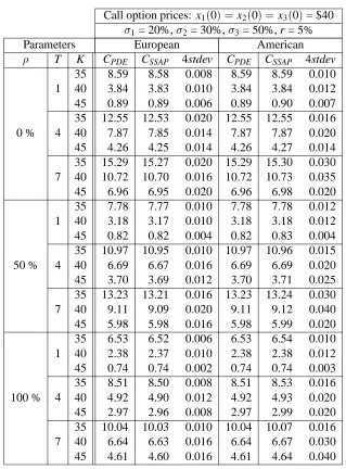
Call option prices: x1(0)= $40, r = 5%
Parameters European American
1 T K CBS CSSAP 4stdev CBS CSSAP 4stdev
35 5.15 5.15 0.001 5.15 5.15 0.002 1 40 1.00 1.00 0.006 1.00 1.00 0.008 45 0.02 0.02 0.001 0.02 0.02 0.001 35 5.76 5.76 0.003 5.76 5.76 0.005 20 % 4 40 2.16 2.16 0.006 2.16 2.16 0.008 45 0.50 0.50 0.004 0.50 0.50 0.004 35 6.40 6.40 0.004 6.40 6.40 0.006 7 40 3.00 2.99 0.010 3.00 3.00 0.010 45 1.09 1.09 0.006 1.09 1.09 0.006 35 5.38 5.38 0.003 5.38 5.40 0.007 1 40 1.91 1.91 0.010 1.91 1.92 0.010 45 0.41 0.41 0.003 0.41 0.41 0.003 35 6.88 6.88 0.010 6.88 6.90 0.020 40 % 4 40 3.96 3.96 0.020 3.96 3.97 0.020 45 2.08 2.08 0.006 2.08 2.09 0.010 35 8.07 8.08 0.010 8.07 8.10 0.020 7 40 5.35 5.34 0.024 5.35 5.36 0.040 45 3.40 3.40 0.012 3.40 3.42 0.020
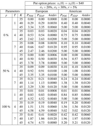
Put option prices: x1(0)= $40, r = 5%
Parameters European American
1 T K PBS PSSAP 4stdev PPDE PSSAP 4stdev
[image:31.612.150.433.95.620.2]35 0.00 0.00 0.001 0.00 0.00 0.001 1 40 0.83 0.83 0.008 0.84 0.84 0.008 45 4.84 4.84 0.001 5.00 5.00 0.000 35 0.19 0.19 0.003 0.19 0.19 0.004 20 % 4 40 1.50 1.50 0.006 1.56 1.56 0.010 45 4.77 4.77 0.004 5.06 5.07 0.010 35 0.41 0.41 0.003 0.42 0.42 0.006 7 40 1.86 1.86 0.010 1.96 1.96 0.012 45 4.82 4.82 0.006 5.24 5.23 0.016 35 0.24 0.24 0.003 0.24 0.24 0.003 1 40 1.74 1.74 0.010 1.75 1.76 0.010 45 5.23 5.23 0.003 5.27 5.29 0.015 35 1.31 1.31 0.010 1.32 1.33 0.020 40 % 4 40 3.31 3.31 0.020 3.36 3.37 0.020 45 6.35 6.35 0.006 6.47 6.49 0.015 35 2.08 2.09 0.012 2.12 2.13 0.015 7 40 4.21 4.21 0.020 4.31 4.31 0.016 45 7.12 7.13 0.012 7.36 7.34 0.030
and
8(i;j)2[1;n]
2
;i6=j; kij=ij for n+1 numbers1>0;:::;n >0 and 1=(n 1)1.
Volatilities (i), correlations (), and interest rate (r) are counted in percent per year. The time to expiration T is counted in months, with the convention 1 month= 30 days. All asset and strike prices are counted in dollars.
Since SSAP uses Monte Carlo simulation, we report confidence intervals together with all results. These confidence intervals are computed from the central limit theorem, i.e. we assume that at a confidence level of 99:95%, the error must be less than 4 times the observed standard deviation of the result. The confidence interval reported is 4stdev.
All the simulations were run on a DEC 3000 model 500X workstation, with an ALPHA AXP processor running at a clock rate of 200 Mhz, and 1 Gigabyte of main memory.
8.2 One underlying asset
We first study the one-dimensional case. In this case, the SSAP price should converge toward the theoretical arbitrage price when both the number of time steps d and the number of cells k converge towards infinity. Both European calls and European puts can be priced according to the original Black-Scholes formula. These prices are reported in the columns European CBS and European PBS of table (1). The American call can also be priced according to the same formula, since we assume the underlying asset pays no dividends. The price is reported in column American CBS. For the American put, we computed the price using the finite-difference method presented in section (4.2). We call this method PDE, since it consists in solving a Partial Differential Equation. In dimension 1, it is essentially equivalent to the Cox-Ross-Rubinstein binomial lattice method. We used 120 time steps for T (time to expiration) ranging from 1 to 4 months, and 210 time steps for T = 7 months. The corresponding price is reported in column American CPDE. The SSAP prices where computed using M=100;000 samples, and k=100 buckets. The number of time steps was set to d=10 in all the experiments.
The observed differences between the SSAP prices and the reference prices are below 0.7%. The confidence interval values are below 1% of the reference prices. American put prices given by the SSAP method are very accurate even when the difference with the European put prices are important (up to 30 cents). The computation time of a price using the SSAP method is about 21 seconds, compared with less than one second with a classical integration method (PDE). In dimension 1, classical finite difference of binomial lattice methods should be preferred to the SSAP method.
8.3 Two underlying assets
Call option prices: x1(0)=x2(0)= $40 1= 20%,2= 30%, r = 5%
Parameters European American
T K CPDE CSSAP 4stdev CPDE CSSAP 4stdev
35 6.80 6.79 0.010 6.80 6.80 0.012
1 40 2.10 2.11 0.002 2.10 2.11 0.002
45 0.18 0.18 0.003 0.18 0.18 0.003
35 8.90 8.89 0.010 8.90 8.90 0.010
0 % 4 40 4.48 4.48 0.015 4.48 4.49 0.015
45 1.66 1.66 0.006 1.66 1.66 0.008
35 10.43 10.42 0.020 10.43 10.43 0.020
7 40 6.15 6.15 0.016 6.15 6.16 0.020
45 3.10 3.08 0.004 3.10 3.09 0.010
35 6.36 6.35 0.004 6.36 6.36 0.005
1 40 1.87 1.87 0.006 1.87 1.87 0.008
45 0.17 0.17 0.004 0.17 0.17 0.004
35 8.09 8.08 0.015 8.09 8.09 0.016
50 % 4 40 3.99 3.98 0.010 3.99 3.99 0.010
45 1.51 1.50 0.006 1.51 1.51 0.006
35 9.41 9.40 0.015 9.41 9.41 0.015
7 40 5.48 5.47 0.010 5.48 5.47 0.016
45 2.77 2.77 0.010 2.77 2.78 0.012
35 5.61 5.61 0.002 5.61 5.61 0.006
1 40 1.45 1.45 0.008 1.45 1.46 0.008
45 1.16 1.16 0.002 1.16 1.16 0.003
35 6.69 6.68 0.003 6.69 6.69 0.008
100 % 4 40 3.09 3.07 0.010 3.09 3.08 0.012
45 1.24 1.24 0.004 1.24 1.25 0.010
35 7.62 7.61 0.006 7.62 7.62 0.012
7 40 4.23 4.21 0.020 4.23 4.22 0.020
[image:33.612.134.447.151.582.2]45 2.24 2.22 0.012 2.24 2.23 0.020