AN ENHANCED RULE APPROACH FOR NETWORK INTRUSION DETECTION USING EFFICIENT DATA ADAPTED DECISION TREE ALGORITHM

(1)

ANALYSIS ON THE DIFFERENT PLASTIC REGION

BETWEEN 2D AND 3D MODEL IN UNDERGROUND

CAVERNS EXCAVATION

1,2_{CHUNHUA YOU,}3_{FANG HAN}

1

School of Civil Engineering, Wuhan University, Wuhan430072, Hubei, China

2

Department of Civil Engineering, Hunan Institute of Technology, Hengyang 421008, Hunan,China

3_{School of Science, Wuhan University of Science and Technology, Wuhan430081, Hubei, China}

ABSTRACT

Analysis and calculation in underground caverns excavation is absolutely a complex three-dimensional (3D) problem, but a two-dimensional (2D) model is usually applied to substitute for the 3D model because of the limit of computer speed and the complexity of the FEM 3D grids. This paper discusses the difference of this two models on the basis of Drucker-Prager yield criteria and the reason why the plastic region from 3D finite element model is smaller than that from 2D model is analyzed in theory. At last, comparative analysis based on the classical FEM software ABAQUS is constructed. The conclusion intuitively shows that the plastic region of 2D model is bigger than that of 3D model, so it is suggested that the 3D finite element model should be built as far as possible in order to describe the plastic region accurately.

Keywords:Underground Caverns, Plane Strain, Three-dimensional Model, Plastic Region, Model Updating

1. INTRODUCTION

There has been great and rapid progress in underground geotechnical engineering and it has expanded the living space of human. With the geotechnical knowledge people can be able to make better use of the resources. Although it has developed for rather a long time, the analysis and design is extremely difficult because of the complexity and uncertainty of the underground geotechnical engineering[1,2]. Usually, there is much difference between the theory and practice, so it is important to study the underground geotechnical engineering for both theory and practice. In future, there will be a long time to go in the underground geotechnical engineering.

The key problem of the underground geotechnical engineering is the stability of the surrounding rock[3,4]. The distribution, size and depth of the plastic region are the most important evidence of the stability of the surrounding rock, which decide the design of the excavation sequence and supporting scheme. The analysis and calculation on the underground caverns excavation is absolutely a complex three-dimensional problem, but a two-dimensional model is usually applied because of the limit of computer complexity and the complexity of 3D grids[5]. In this way the plastic region obtained from 3D model is extremely

different from the region obtained from the 2D model. Project[6,7] shows that the plastic region obtained from 2D model simplified as plane strain problem is bigger than the real 3D model.

In fact, the underground caverns excavation problem is not strictly satisfy the plane strain assumption[8], so it is not appropriate to simplify the 3D model as the 2D model. In this paper, the difference of the two models on the basis of Drucker-Prager yield criteria is discussed with the material nonlinearity and the reason why the plastic region from 3D finite element model is smaller than the plastic region from 2D model is analyzed in theory.

2. YIELD FUNCTION

When analyzing the plastic region of the underground caverns excavation under the action of ground stress, consider the initial ground stress as the three-directional pressure based on the Drucker-Prager yield criteria in the 3D model[9,10]. Drucker-Prager yield criteria is based on the Mohr-Coulomb criteria, and fit to rock and soil materials. At present, the study and application of Drucker-Prager yield criteria are classical Drucker-Drucker-Prager yield criteria[11]. The yield function on the meridional plane is written as follows:

k

J

I

(2)

ISSN: 1992-8645 www.jatit.org E-ISSN: 1817-3195

Where

f

is the yield function,

I

₁ is the first

stress invariant and

J

₂ is the second deviatoric

stress invariant. Parameters

α

and

k

denote the positive material constants[12].

In real 3D model, the parameters

α

and

k

are calculated as follows:

( )

) sin 3 ( 3 sin 2 3

φ

α

− =

D

( )

) sin 3 ( 3 cos 6 3

φ

− = C

k _D (2)

In 2D model simplified as plane strain problem, when the Drucker-Prager yield criteria is consistent

with the Mohr-Coulomb criteria, the parameters α

and k are calculated as follows:

( )

φ

α

2 2

tan

12

9 tan

+

=

D

( )

φ

2 2 tan 12 9 3 + = C k D (3)

Where

C

is the soil cohesion and

φ

is the

internal friction angle both in Eq.(2) and Eq.(3). When analyzing the elastic and plastic region with the incremental method, the state of the element may be the following three kinds of cases:

(1)Elastic element: the element is elastic at the 1

i− incremental step and will be elastic at the

i

incremental step, so the relations

{ } { }

σ i = σ i−1+

[ ]

De

{ }

∆ε i andf(

{ }

σ i)<0 are established.

(2)Plastic element: the element has come to plastic at the

i

−

1

incremental step which means

{ }

( _i) 0

f σ = and the element will also be plastic at

the

i

incremental step which can also be written

asf

(

{ }

σ _i

)

=₀.

(3)Elastic-plastic transition element: the element is elastic at the end of the

i

−

1

incremental step which means ₍

{ }

₎_<₀

i

f σ and it will come to plastic

at the

i

incremental step, written as

(

{ }

)

₌₀

i

f σ .

For different states, such as elastic element and the elastic-plastic transition element, the 3D and 2D model will use different formulas:

For 2D model simplified as plane strain problem:

( )

1 2

1 2 1 2

( )

x y x y

D

I

σ

µ σ

σ

σ σ

µ σ σ

= + + +

= + + + (4)

( )

(

)

(

)

(

)

(

)

2 2

1 2 2 1

2 2 2

2 1

1 1

6 ₁

D

J σ σ µ σ µσ

µσ µ σ

 ₋ ₊ ₋ ₋    = ₊ _{− −}    (5)

For 3D model:

( )

1 3

1 2 3

x y z

D

I

σ

σ σ

σ

= + +

= + + (6)

( )

(

) (

)

(

)

2 2

1 2 2 3

2 3 2

3 1

1 6 D

J σ σ σ σ

σ σ  − + −    = + −    (7)

For the plastic element in the 2D plane strain model:

( )

1 2 1 2

( )

2 2 2

3

( ) 3 ( )

2

plastic

D

D D

I = σ σ+ − α J (8)

2 1 2

2 2 2

2

( )

4(1 3( ) )

plastic D

D

J σ σ

α − −

＝ (9)

For the plastic element in 3D model, the formulas are the same as Eq.(6) and Eq.(7).

The yield functions describing the Drucker-Prager yield criteria are shown as follows:

Elastic element (2D):

( )

2 2 1 2 2 2 2

(f D elastic) =( )

α

D I D+ J D−( )k D (10)

Elastic element (3D):

( )

3 3 1 3 3 3 3

(f D elastic) =( )

α

D I D+ J D −( )k D (11)

Plastic element (2D):

( )

2 2 1 2 2 2 2

( _D)_plastic ( ) _D plastic plastic ( )_D

D D

f = α I + J − k (12)

Plastic element (3D):

( )

3 3 1 3 2 3 3

( _D)_plastic ( )_D plastic plastic ( )_D

D D

f = α I + J − k (13)

In conclusion, for 3D model the yield functions are the same, written as

(

f

₃_D

)

_plastic

=

(

f

₃_{D elastic}

)

, on the contrary, for 2D model the yield functions are different, written as

(

f

₂D

)

plastic

≠

(

f

₂D

)

plastic, so the

property of the element whether it is elastic or plastic should be considered if the 2D plane strain model is used.

3. COMPARATIVE ANALYSIS

For further analysis, separate the yield function into two parts. Part one is

α

I₁+ J₂ and part two

is

k

. If

α

I1+ J2 <k, that is f <0, the element is elastic, on the contrary, if

α

I

₁

+

J

₂

=

k

, that isf =0, the element is plastic.

First compare the

k

part with 2D and 3D model. The following formula can be obtained from Eq.(2) and Eq.(3):

3 2 ₂

2

6 cos 3

( ) ( )

3(3 sin ) 9 12

2 cos 1

3

3 sin 3 4

(3)

If ₀o _<φ_<₉₀o_{, formula}

2

2 cos 1

3 sin _{3 4}_tg

φ

φ> _φ

− ₊

is

established, so ₍_k₃_D₎>₍_k₂_D₎.

Then compare the

α

I

₁

+

J

₂ part with 2D and

3D model. Let

2 2 2 2

( ) ( )plastic ( )plastic

D D D

A=

α

I ＋ J and

D D

D I J

B=(

α

)3 ( )3 ＋ ( 2)3 , expand the

parameters

A

and

B

respectively as follows:

2 2 2 1 2 1

2 ₍ ₎ ₁ ₃₍ ₎

2 1 2 ) ( ) ( 3 D D

A= α σ +σ + σ −σ − α (15)

1 2 3

2 2 2

1 2 2 3 3 1

2 sin

( )

3(3 sin )

1

( ) ( ) ( )

6

B φ σ σ σ

φ

σ σ σ σ σ σ

= + + +

−

 − − − − − 

 

(16)

Considering the three-directional pressure of the underground caverns excavation in real project, the order of magnitude of the two normal stress in horizontal direction is equivalent, but the normal stress in vertical direction is not equivalent as there exists a scale factor

β

. For 2D plane strain model, let

σ

₁ =−

σ

₀and

σ

₂

=

−

βσ

₀. The stress status of the corresponding 3D model is

σ

₁

=

σ

₂

= −

σ

₀ and

0

3

βσ

σ

=

−

. Take the parameters into Eq.(15) and

Eq.(16):

[

β φ β φ

]

φ

σ 2

2

0 ₍₁ ₎ ₁ ₁

4 3 2 3 tg tg tg

A + − − +

+ − = (17) 0 1 3 1 ) sin 3 ( 3 sin ) 2 (

2 _β _σ

φ φ β       − + − + − = B (18)

(1) When

β

>1, let T=

(

A−B

)

σ0, then

(

2

)

2

3 1

(1 ) 1 (1 )

2 _{3 4}

1 2(2 ) sin

( 1)

3 3(3 sin )

T tg tg

tg

β φ φ β

φ β φ β φ = − + + + − + + − − + − (19) 2 2 3 1

( 1 )

2 _{3 4}

3(1 sin ) 3 sin T tg tg tg φ φ β _φ φ φ ∂ _{= −} ₋ ₊ ∂ ₊ − − − (20) 2 2 2 3 2 (1 ) 3 1

3(1 ) 1

2 (3 4 )

3 cos (4 2 )

(3 sin )

tg tg T tg tg β φ φ

φ φ β φ

φ β φ − −   + ∂ _{= −} _ _   ∂ +  + +  + + − (21)

If o

90

0<

φ

< , the relation ∂ ∂ <T β 0is derived with the software Matlab as shown in Fig.1. If

o o

90

20 <φ< and 1<β <5, the relation ∂ ∂ >_T φ ₀ is derived as shown in Fig.2.

Figure 1 The Curve Of∂ ∂T β

Figure 2 The Curve Of T∂ ∂φ

From the curves above (Fig.1 and Fig.2) it can be derived that for

T

(

β

=

3 ,

φ

=

30

o

)

=

0

, then

0 ) 90 ~ 30 , 3 ~ 1

( = = o o >

T

β

φ

.

(2) When

β

<

1

, let S=

(

A−B

)

σ₀, then

(

2

)

2

3 1

(1 ) 1 (1 )

2 _{3 4}

1 2(2 ) sin

(1 )

3 3(3 sin )

S tg tg

tg

β φ φ β

(4)

ISSN: 1992-8645 www.jatit.org E-ISSN: 1817-3195

2

3 1

(

2 _{3 4}

3 sin

1 )

3(3 sin )

S

tg tg

tg

φ

β _φ

φ φ

φ

∂

= − +

∂ ₊

+

+ +

−

(23)

2

2 2 3

2

(1 ) 1

3

2 (3 4 ) 3(1 ) 1

3 cos (4 2 ) (3 sin )

tg tg

S

tg tg

β φ φ

φ φ β φ

φ β

φ

− +

 

+

∂ _{= −}

 

∂ + _ + + _

+ +

−

[image:4.612.94.452.75.632.2]

(24)

Figure 3 The Curve Of ∂ ∂S β

Figure 4 The Curve Of

∂ ∂

S

φ

If o

90

0<

φ

< , the relation ∂ ∂ >S β 0is derived

as shown in Fig.3. If o o

90

20 <φ< and 1<

β

<5, the relation∂ ∂ >S φ 0 is derived as shown in Fig.4.

From the curves above (Fig.3 and Fig.4) it can be derived that for S(

β

=0.1,

φ

=13o)≈0.0577, then

0 0577 . 0 ) 90 ~ 13 , 1 ~ 1 . 0

( = = o o > >

S

β

φ

.

From all above, if 0.1<

β

<3 and

o o

90

30 <

φ

< , then

T

>

0

and

S

>

0

, in other

words , if

0 .

1 <

β

<

3

and o o

90

30 <

φ

< , then

B

A

>

. In summary of Eq.(14) to Eq.(16), the

result shows that the plastic region from 2D finite element model is bigger than the plastic region from 3D model in theory.

4. NUMERICAL VERIFICATION

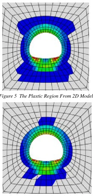
A simulated underground caverns excavation progress based on 2D plane strain model and 3D model are considered to demonstrate the expansion procedure of the plastic region based on the software ABAQUS as shown in Fig.5 and Fig.6.

The results indicate that the plastic region from 2D model is obviously bigger than the region from 3D model. The plane strain problem simplified as 2D model will magnify the plastic region, this may induce unnecessary waste and may not be safe.

Figure 5 The Plastic Region From 2D Model

[image:4.612.337.500.358.700.2]

(5)

5. CONCLUSIONS

In this paper, the reason why the plastic region from the 2D plane strain model is bigger than the 3D model is proved in theory based on the classical Drucker-Prager yield criteria, and then a simulated underground caverns excavation progress is derived to verify the conclusion intuitively. It is suggested that the best way to describe the plastic region is to build the 3D model as far as possible, that will be safe and economical.

ACKNOWLEDGEMEN

TS

This work was supported by Science and Technology Commission of Hunan Province (NO.2009SK3034) and National Natural Science Foundation of China (NO.51108358).

REFERENCES:

[1] H.Yoshida, H.Horii, “Micromechanics-based continuum model for a jointed rock mass and excavation analyses of a large-scale cavern”,

International Journal of Rock Mechanics and Mining Sciences, Vol. 41, No.5, 2004, pp.119– 145.

[2] T.Sitharam, G.Latha, “Simulation of excavations in jointed rock mass using a practical equivalent continuum approach”, International Journal of Rock Mechanics and Mining Sciences, Vol. 39, No. 1, 2002, pp.517–525. [3] W.S. Zhu, B. Sui, X.J. Li, S.C. Li, W.T. Wang,

“A methodology for studying the high wall displacement of large scale underground cavern groups and it's

applications”, Tunnelling and Underground

Space Technology, Vol. 6, No. 2 ,2008, pp.651–664.

[4] G.Barla, A.R.Fava, G.Peri, “Design and construction of the Venaus powerhouse cavern

in Calcschists”, Geomechanics Tunnelling,

Vol. 1, No. 1, 2008, pp. 399–406.

[5] S.C.Fan, Y.Y.Jiao, J.Zhao, “On modeling of incident boundary for wave propagation in jointed rock masses using discrete element method”, Computers and Geotechnics,Vol. 1, No. 1, 2004, pp.57–66.

[6] M.Tezuka, T.Seoka, “Latest technology of underground rock cavern excavation in Japan”,

Tunnelling and Underground Space Technology, Vol. 18, No. 3, 2003, pp.127–144.

[7] Y.Jiao, S.Fan, J.Zhao,

“

Numerical investigation of joint effect on shock wave propagation in

jointed rock masses”, Journal of Testing and

Evaluation, Vol. 18, No. 3, 2003, pp.127–144.

[8] G.X.Guo, Y.M.Guo, B.L.Qing, F.C.Zhi,

“Underground excavation in Xiaolangdi

project in Yellow River,” Engineering

Geology, Vol. 76, No. 10 , 2004, pp.129–139. [9] K.R.Dhawan, D.N.Singh, I.D.Gupta,

“Three-dimensional finite element analysis of underground caverns”, International Journal for Numerical and Analytical Methods in Geomechanics. Vol. 4, No.5, 2004, pp. 224– 228.

[10] T.Wang, X.L.Chen, J.Yang, “Study on stability of underground cavern based on 3D GIS and

3D EC”, Chinese Journal of Rock Mechanics

and Engineering, Vol.24, No. 15, 2005, pp.3476–3481.

[11] T.G.Sitharam, G.M.Latha, “Simulation of excavations in jointed rock mass using a practical equivalent continuum approach”,

International Journal of Rock Mechanics and Mining Sciences, Vol. 24, No. 39, 2002, pp.517–525.

[12] T.Wang, X.L.Chen, L.H.Yu, “Discrete element calculation of surrounding rock mass stability

of underground cavern group”, Rock Soil