Trojans in Wireless Sensor Networks

Georgia State University Georgia State University

ScholarWorks @ Georgia State University

ScholarWorks @ Georgia State University

Geosciences Theses Department of Geosciences

Spring 5-10-2014

GIS Least-Cost Route Modeling Of The Proposed Trans-Anatolian

GIS Least-Cost Route Modeling Of The Proposed Trans-Anatolian

Pipeline In Western Turkey

Pipeline In Western Turkey

Austin Kelly

Georgia State University

Follow this and additional works at: https://scholarworks.gsu.edu/geosciences_theses

Recommended Citation Recommended Citation

Kelly, Austin, "GIS Least-Cost Route Modeling Of The Proposed Trans-Anatolian Pipeline In Western Turkey." Thesis, Georgia State University, 2014.

https://scholarworks.gsu.edu/geosciences_theses/71

by

AUSTIN KELLY

Under the Direction of Timothy Hawthorne

ABSTRACT

The routing of the Trans-Anatolian Pipeline plays an important role in the future energy

security of the European Union. The natural gas pipeline is planned to run from the natural gas

fields in the Caspian Sea through Turkey. This project is a case study for a Geographic

Infor-mation System (GIS) least-cost route analysis of a section of the proposed pipeline in Western

Turkey. The route analysis comprised of weighting multiple types of criteria in a compiled risk

assessment map that was analyzed by a least-cost algorithm to display the least hazardous route

through the study area. Multiple varieties of criteria were considered such as, lithology, slope of

terrain, environmental and social risk factors, e.g. proximity to natural reserves and urban

cen-ters, to provide the least hazardous route through the region. The derived least cost paths were

more efficient than the proposed route in the relative cost associated with each route.

GIS LEAST-COST ROUTE MODELING OF THE PROPOSED TRANS-ANATOLIAN

PIPE-LINE IN WESTERN TURKEY

by

AUSTIN KELLY

A Thesis Submitted in Partial Fulfillment of the Requirements for the Degree of

Master of Science

in the College of Arts and Sciences

Georgia State University

Copyright by Austin Godfrey Kelly

GIS LEAST-COST ROUTE MODELING OF THE PROPOSED TRANS-ANATOLIAN

PIPE-LINE IN WESTERN TURKEY

by

AUSTIN KELLY

Committee Chair: Timothy Hawthorne

Committee: Jeremy Diem

Lawrence Kiage

Electronic Version Approved:

Office of Graduate Studies

College of Arts and Sciences

Georgia State University

DEDICATION

I would like to dedicate this thesis to my mother for it was her that taught me everything I

know in life. Without her guidance I would not have become the man I am today. Through the

ups and downs you have always been there to help me persevere and overcome. I cannot thank

v

ACKNOWLEDGEMENTS

I would like to thank all of the Georgia State Department of Geosciences Faculty that

have helped me along the way in this project. I especially would like to acknowledge the support

and guidance of my committee chair and members, Dr. Timothy Hawthorne, Dr. Jeremy Diem,

and Dr. Lawrence Kiage. I would also like to thank the support from all of my friends and

TABLE OF CONTENTS

ACKNOWLEDGEMENTS ... v

LIST OF TABLES ... viii

LIST OF FIGURES ... ix

1 PROJECT SUMMARY ... 1

1.1 Geo-Political Background and Least-Cost Analysis ... 1

1.2 Study Region ... 2

2 INTRODUCTION ... 7

2.1 Purpose of the Study ... 7

2.1.1 Research Questions ... 9

2.1.2 Literature Review ... 10

3 EXPERIMENT ... 15

3.1 Methods and Data ... 15

3.1.1 Accumulated Cost Surface Creation ... 19

3.2 Least-Cost Routing Tool ... 21

4 RESULTS ... 24

4.1 Equal Weighting ... 24

4.2 Weighted Overlay ... 26

4.3 TANAP Proposed Route ... 31

vii

5.1 Trans-Anatolian Natural Gas Pipeline Least-Cost Analysis ... 34

5.2 Limitations of this Route Model ... 38

6 CONCLUSION ... 40

LIST OF TABLES

Table 1. Least-Cost Path and Straight-Line Path lengths in km and relative cost values

using the Equal Weighted Cost Surface. GCS: WGS-84, Projection: Lambert Conformal

Conic. ... 25

Table 2. Weight Percentages for each criterion in all 3 Weighted Overlay Cost Surfaces. . 26

Table 3. Least-Cost Paths and Straight-Line Paths for each of the specified Weighted

Overlay Cost Surfaces. Detailed lengths in km and relative cost values for each path on

the respected cost surface. GCS: WGS-84, Projection: Lambert Conformal Conic. ... 30

Table 4. Detailed length in km and relative cost for proposed TANAP route through each

separate cost surface. Does not include connection from Canakkale to

Tekirdag-Bulgarian border. GCS: WGS-84, Projection: Lambert Conformal Conic. ... 32

Table 5. Error polygon areas between each created route and the proposed TANAP route.

ix

LIST OF FIGURES

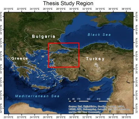
Figure 1. Red rectangular outline details the thesis study region and the maximum extent

of the cost accumulated surfaces. ... 3

Figure 2. Slope criterion raster for the study region where red areas equal areas of high

risk and green areas equal areas of low risk. Areas of zero slope have also been included

in the areas of high risk as they indicate water bodies. ... 4

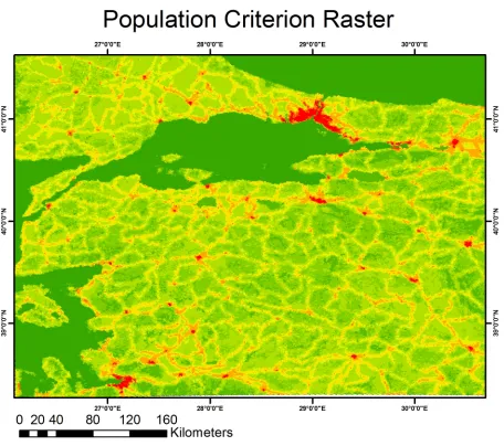
Figure 3. Population criterion raster representing the population density throughout the

study region. Red areas indicate areas of high population density and green areas

represent areas of low population density... 5

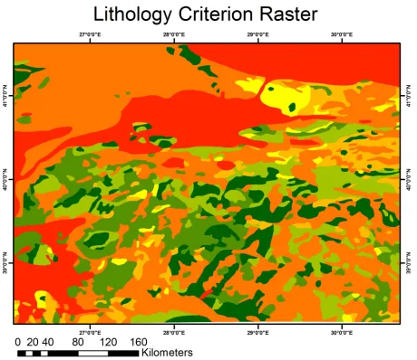
Figure 4. Lithology criterion raster displaying the different lithologic units within the study

area. Red indicates units of high risk and green represents areas of low risk. ... 6

Figure 5. Proposed TANAP route overlain onto the slope raster of the study area. Route

was compiled by Cindar Engineering and Consulting Inc. ... 7

Figure 6. Process used to format each individual criterion into a continuous raster surface,

and then combine those factor rasters into a cost surface. This info graphic details the

process for the Equal Weighted Cost Surface. For the Weighted Overlays each factor

raster was designated a specific weight percentage using the Weighted Overlay tool

within ArcGIS, otherwise the main steps are identical... 23

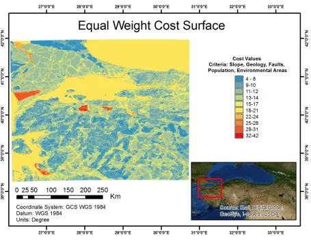
Figure 7. Equal Weight cost surface that was created for the study area. It was from this

surface that the least-cost path was derived. ... 24

Figure 8. Least-cost route and straight-line path that was created for cost surface Equal

Figure 9. Least-cost route and straight-line path that was created for cost surface Weighted

Overlay 1. ... 28

Figure 10. Least-cost route and straight-line path that was created for cost surface

Weighted Overlay 2. ... 29

Figure 11. Least-cost route and straight-line path that was created for cost surface

Weighted Overlay 3. ... 30

Figure 12. Displays the least-cost routes derived from all 4 cost surfaces and the proposed

1

1 PROJECT SUMMARY

1.1 Geo-Political Background and Least-Cost Analysis

The geo-political tensions between Russia and the European Union (EU) over the routing

of newly discovered Caspian gas from Azerbaijani, Turkmen, and Iranian fields is a current topic

of great importance in European Union energy security. The Trans-Anatolian natural gas

pipe-line (TANAP) aims to connect Caspian Sea natural gas to Southeastern Europe via Turkey. This

pipeline will allow the EU freedom from Russian and Ukrainian gas sources, which have

plagued the European Union in recent decades by controlling prices and limiting the supply to

the continent (Erdogdu 2010; Varol Sevim 2013; Stern 2006). This study demonstrated a

strate-gic GIS least-cost routing analysis of a determined geographic area through which a section of

the pipeline will pass through Western Turkey. The route model determined the most

economi-cally and environmentally safe route through the given geographical area by taking into

consid-eration geological, environmental, and social hazards. By incorporating these multiple criteria

(lithology, slope, population density, environmentally sensitive areas, and geologic hazards) this

study provides a case study for which future large-scale projects can plan simultaneously, the

most economical and least hazard prone route.

Major criteria that were considered in the GIS analysis are geologic factors such as,

li-thology, proximity to faults, slope, and landslide susceptibility. These factors were implemented

alongside environmental and social factors such as: proximity to water bodies, proximity to

dense urban areas, and the proximity to areas of high biodiversity. The data was compiled

through multiple sources such as United States Geological Survey (USGS) databases, EuroStat,

dis-playing physical features of the region. The methodology used to determine this model was

ref-erenced from multiple scholarly articles and includes the use of the ESRI ArcGIS Cost Path tool.

All criteria were compiled into an ArcGIS geodatabase and rasterized to be given a specific

haz-ard weight. Each criterion’s weight factor was combined together through the use of a Boolean

query to provide a risk assessment map of the geographical study area, which was then used by

the Cost Path tool specified earlier to produce the best route. The final result included multiple

route maps of the planned pipeline displaying the most economical and least hazardous route

through the specified geographic study area and provided an innovative new case study to further

advance Geographic Information Science by incorporating both physical and environmental risk

factors.

1.2 Study Region

The study region for this thesis is shown in Figure 1 below and covers an area of 150,960

square kilometers. The study region is located in Northwestern Turkey and includes the major

metropolis of Istanbul and the Sea of Marmara. This area represents the extreme western portion

of the Trans-Anatolian Pipeline where it will eventually connect to other major pipelines on the

Greece-Turkey border and Bulgaria-Turkey border. The economic hub of Istanbul and the major

shipping lane from the Black Sea to the Mediterranean via the Turkish Straits are located within

this region. This congested and vital shipping lane is one key reason why this area was chosen

for this thesis.

This shipping lane handles enormous amounts of tanker traffic moving both oil and

natu-ral gas from Russian ports on the Black Sea coast to the Mediterranean to be sold in Western

Eu-rope. The TANAP Project plans to alleviate some of this traffic through the straits by bypassing

3

Figure 1. Red rectangular outline details the thesis study region and the maximum extent of the cost accumu-lated surfaces.

Within this study region extent each of the criterion rasters were created. Figures 2

through 4 display the criterion rasters for three of the five criteria that were assessed in this

the-sis. The criterion rasters display the reclassified values for each raster where the red locations

correspond to the areas of highest risk for that specific criterion and areas of green correspond to

areas of lowest risk. The color spectrum for these figures indicating highest risk to lowest risk is

5

Figure 4. Lithology criterion raster displaying the different lithologic units within the study area. Red indi-cates units of high risk and green represents areas of low risk.

As of March 2013 the proposed route of the TANAP project was compiled by Cindar

Engineering and Consulting Inc and displayed in Figure 5 (“Environmental Independent

As-sessment Application” 2013). This proposed route of the pipeline was used to compare the least

cost paths that were created to determine their validity. More detail on this proposed route will

7

Figure 5. Proposed TANAP route overlain onto the slope raster of the study area. Route was compiled by Cindar Engineering and Consulting Inc.

2 INTRODUCTION

2.1 Purpose of the Study

With its already high demand for natural gas set to increase in the next few decades, the

European Union is at a crossroads in determining from where it will import its natural gas

(Omonbude 2009). At the current state, Russia accounts for the largest exporter of natural gas to

the European Union, as it holds the world’s largest natural reserves and is conveniently located

geographically to the east. The easiest and most economical transport routes and techniques

locat-ed around the Caspian Sea and more recently the Yamal Peninsula to markets in Europe

(Gazprom 2011). Liquefied Natural Gas (LNG) transported through the use of specific LNG

tanker ships offers the other main option to transporting natural gas but due to extremely high

costs of refining and construction of LNG terminals the pressured pipeline transport remains the

most favorable. These LNG tankers also pose a specific problem for this particular route due to

the chokepoint that occurs within the Turkish Straits and therefore are not considered to be a

via-ble option (Cemal&Güven et al. 2008; Bolat and Yongxing 2013). The Russian natural gas

pipe-lines are primarily routed through the country of Ukraine to provide the quickest access to main

gas terminals in Central Europe. In the past decade numerous disputes over transit fees and the

pricing of gas through these pipelines led the Russian government to shut off the supply of gas

resulting in massive shortages throughout Europe (Stern 2006). This high profile political

inci-dent led the leaders of the European Union to begin to diversify their imports of natural gas from

other markets in order to have stable sources of natural gas (Guili 2008; Baev and Øverland

2010). Recent discoveries of large natural gas fields in the Caspian region in Azerbaijan,

Turk-menistan, and Iran have become the focus of European leaders, with the main route of transit

be-ing through the Anatolian Peninsula (Varol Sevim 2013; BP Exploration Ltd. 2013). The most

prominent project that is being proposed is the Trans-Anatolian Pipeline linking the Caspian gas

fields to the transit pipelines in Southeastern Europe (Erdogdu 2010). This pipeline will

eventu-ally have the capacity to transport up to 60 billion cubic meters (bcm) of natural gas per year into

the European Union and bypassing Russia and Ukraine completely (“TANAP – Trans Anadolu

Doğal Gaz Boru Hattı Projesi | 2 Devlet, Tek Millet!” 2014).

This thesis addressed the next key phase in the Trans-Anatolian Pipeline production,

rout-9

ing of this pipeline is of great importance in the final investment costs of the project due to the

fact that pipelines are static infrastructure features and are therefore more susceptible to damage

from natural hazards. The costs of pipeline failures, both financially and environmentally, are

enormous and can easily shut down a project like TANAP (Brody, Bianca, and Krysa 2012;

Hindery 2004; Yang et al. 2010). Thus, the GIS analysis of the region and the use of this analysis

to determine the least hazardous and most cost effective route are of great importance to the

completion of the pipeline. The least-cost route model that was developed through this project

displays more efficient routes for the Trans-Anatolian Pipeline through this region based on the

most readily available data for each specific criterion.

It is pertinent to point out that in this study the “least cost” route is designated by the least

hazardous route across the physical features of where the pipeline will be located not the

con-struction costs of these locations. The calculated cost value of the route by the model should be

regarded as relative to the costs associated with the pipeline in the long term.

2.1.1 Research Questions

There are three research questions that were answered with the development of this

rout-ing model. They are as follows:

1) What is the least hazardous route for the Trans-Anatolian Pipeline through the study

region within Western Turkey?

2) What criteria are the most influential in costs of routing this pipeline?

3) When comparing the official proposed route to the experimental results of this thesis,

2.1.2 Literature Review

Large-scale linear projects, such as natural gas pipelines, are planned and designed

around a concise route to limit the costs and materials of production. The most efficient process

to determine this route is through the use of GIS and a least-cost routing model (Aissi, Chakhar,

and Mousseau 2012; Rees 2004; Feldman et al. 1995). Current GIS techniques allow for large

amounts of cost-analysis data to be collected, stored, and analyzed and thus improve the route

accuracy for large-scale projects (Luettinger and Clark 2005). Through the research of multiple

studies such as, Feldman et al. 1995 and Saha et al. 2005, the methodology was formulated to

create these least cost models for various criteria evaluations and to incorporate multiple criteria

into one least cost model. The complexities of the least cost model have limited the categories of

criteria that have been examined. Most of the criteria examined have been physical

characteris-tics of the given geographic area due to the more straightforward approach to weighting the

vari-ations of a specific factor (Atkinson et al. 2005; Collischonn and Pilar 2000; Saha et al. 2005;

Aissi, Chakhar, and Mousseau 2012). Very few studies have included the biological impacts

when determining the routing of a pipeline and included those criteria into the model. One,

Lovett et al. 1997, used a least cost model to route hazardous waste through specific paths and

provided a risk assessment due to biological hazards such as population and environmental risk

(Lovett, Parfitt, and Brainard 1997).

Questions on how to develop a process to determine the shortest and least costly routes

have had scholars analyzing different techniques for many years. One of the first academics to

provide a solution to the problem was Edsger Dijkstra who developed an algorithm to determine

the shortest path between two points connected in a network (Dijkstra 1959). This algorithm is

cost-11

accumulated surface the algorithm is able to selectively choose the least costly route through a

given area. This type of analysis focuses on the neighborhood of cells around the proposed

start-ing location and moves outward from that location to eventually encompass the entire study area.

There are many types of patterns that the algorithm can take to create the cost accumulated

sur-face, with each different pattern offering a different approach to solve the problem at hand

(Iqbal, Sattar, and Nawaz 2006; Luettinger and Clark 2005). The Dijkstra Algorithm is one of

the most commonly used tools to determine the least cost route through a surface and one of the

simplest methods. This is due to the fact that once all of the criteria are compiled together into a

cost accumulated surface the algorithm need only analyze the nodes across the surface. One

limi-tation, however, to using this type of algorithm is that it is computationally demanding and

pro-duces large amounts of data to be stored (Saha et al. 2005).

In order to improve on this computationally demanding process that was used more and

more companies began to develop new GIS extension packages to limit computation time and

also expedite results. The Environmental Systems Research Institute (ESRI) extension,

PATHDISTANCE, uses a smaller scale neighborhood analysis in order to try and control the

ef-fects of the model and make the path created more realistic (Saha et al. 2005). In effect the use of

this smaller scale would make the compiled path less erratic and much more smooth. This is key

when planning pipeline route design due to the fact that a pipeline is connected together much

more rigidly than, say, a road. Extensions, such as PATHDISTANCE, became much more

prom-inent in studies due to their accessibility and this option to create much smoother designs.

Alt-hough their downside was that the limitation of the neighborhood analysis meant they could not

accurately predict points in mountainous areas (Saha et al. 2005). The rapidly changing

of the route to be determined. Therefore for these types of areas alternative methods must still be

applied. In recent years ESRI has developed more complex cost path extensions and included

them in their main ArcGIS products. One of these extensions that have been of significant use is

the Cost Path tool. This tool allows for the creation of both a Cost Direction surface as well as a

Backlink surface that are then used alongside the main Cost surface to determine a more accurate

and precise Cost Path from a source point to a destination point, all the while calculating the cost

that the path acquires across the surface (Collischonn and Pilar 2000; Rees 2004).

Real world case studies have been performed to determine the least cost routes of major

pipelines and are mainly funded by major operators in the industry. In the studies researchers

uti-lize both remotely sensed and GIS data to develop the necessary criteria for analysis. The

Bechtel Corporation in its analysis to develop a route for a proposed pipeline in the Caspian Sea

region provided one such case study. The researchers factored in criteria from the terrain, land

use, geology, etc. through the use of geospatial data sets (Saha et al. 2005; Feldman et al. 1995).

The use of remotely sensed data allows for areas all over the globe to be examined and evaluated

without the researchers physically traveling to the specified location. The costs associated with

the construction in each specific criterion were determined from a previous study that was

un-published by Bechtel, allowing the researchers to obtain a greater accuracy on the actual real

world costs. Factoring into these costs were also the environmental and future liability costs

should the pipeline be located within areas that were deemed likely for future hazards to occur,

e.g., close proximity to faults, river/stream crossings (Feldman et al. 1995). Feldman et al. 1995

is one of the first studies to actively integrate these types of criteria into the least cost routing

model due to the availability of remotely sensed and previously researched cost data. Through

13

the straight line path but 14% less costly to construct (Feldman et al. 1995). This offers a case

where the least cost route can be examined efficiently through the use of geospatial data.

View-shed analysis offers another approach to determine the least costly routes through a

specified area (Lee and Stucky 1998). The same general methodology that is discussed earlier in

this thesis is used in creating a cost accumulated surface and a least cost algorithm or program

extension is used to calculate the least costly route through that surface. In using view-shed

anal-ysis by Lee and Stucky 1998 a digital elevation model (DEM) was used to 4 select types of paths

through the study area based on visibility. While this model is useful for environmental planning

and civil engineering, when tested for pipeline construction, the analysis returned results that

were infeasible for construction (Lee and Stucky 1998). This specific study also did not factor in

other factors that would have accounted for this problem such as geology, terrain, and land use

(Saha et al. 2005; Lee and Stucky 1998). Therefore for pipeline routing and the focus of this

the-sis, view-shed analysis was not incorporated into the methodology when developing the least

cost path for TANAP.

Other studies that have been done more recently focus on the costs of crossing water

bod-ies and the built environment (e.g. roads, bridges, etc.) and on the slope of the terrain (Iqbal,

Sattar, and Nawaz 2006). The area analyzed in the research by Iqbal et al. 2006 was again in a

very mountainous region of northern India, where the changing gradient of the terrain in short

distances played a key part in determining where a pipeline could be located. The criteria that

were analyzed were first reclassified through a Spatial Decision Support System (SDSS) in order

to make the entire system more result oriented and simpler to process (Iqbal, Sattar, and Nawaz

2006). The result of the study displayed that while the least cost route was 1 km longer than the

accurately displayed a more economical route and can be integrated into many other fields such

as the planning of water/sewer pipelines which also require economical route planning (Iqbal,

Sattar, and Nawaz 2006).

Other linear features similar to natural gas pipelines that have used least-cost routing

models to more accurately plan economic routes are roads and canals. With these features the

impact of topography is very important, especially in canals, and influences the cost accumulated

surface by making the weighting values direction dependent. With this specific requirement the

algorithm used to process the cost accumulated surface must be adapted to accommodate this

restriction (Collischonn and Pilar 2000). This type of restriction seems to be more prevalent in

areas where the topography is fairly consistent due to the fact that the algorithm must employ a

function describing the slope into its calculations.

These past studies have employed methodologies to obtain the same result of a thin route

that is created by linking individual cells from the cost accumulated surface together from the

starting point to the destination. The process of also incorporating a specified path width to the

route selection process is advantageous when the proposed route is required to be wider than one

of the raster cells used in the cost accumulated surface (Gonçalves 2010). This method of routing

uses an adapted algorithm with a larger moving window to incorporate the expanded route width.

This type of routing can drastically alter the most economical route through a surface due to the

restricting parameters but allows planners to develop routes that include specific sizes of

ease-ments or right of ways that accompany most major projects, especially pipelines (Gonçalves

2010). With this type of routing planners are able to incorporate right of way distances into their

15

This review clearly demonstrates the multitude of applications that GIS based least cost

routing has in the planning of major linear projects. Past and current developments through

up-dating algorithms and applying more diverse criteria into a cost accumulated raster allow least

cost routing extensions in multiple GIS platforms to efficiently assess the criteria and display the

most economical and least hazardous route through a given geographical area. New

advance-ments in GIS and remote sensing technology have allowed researchers to incorporate multiple

categories of data such as topographic, environmental, and geological data to more accurately

and realistically predict the costs associated with routing linear features such as natural gas

pipe-lines.

3 EXPERIMENT

3.1 Methods and Data

In order to apply least-cost routing models to an area, geospatial datasets are required to

assess the multiple criteria that will be evaluated. These maps need to be of a high enough

reso-lution to accurately display the changing topographic and geologic features in the area. In this

area of Western Turkey the Digital Elevation Model (DEM) that was used was downloaded from

the NASA JPL Shuttle Radar Topography Mission (SRTM) and had a resolution of 90m cell

size. This DEM and resolution was used due to its availability to cover the entire study region

and keep the storage size of the raster files low. Due to the large geographic extent of the study

region a finer resolution DEM would have created large raster file sizes that are not easily

ma-nipulated within ArcGIS. The DEM scenes were mosaicked together in one continuous raster

surface covering the entire study area using the Mosaic tool in ArcGIS. Sinks and holes in the

play more accurate results This filled DEM surface was then used to create a criterion raster

dis-playing the slope of the terrain over the geographic area that was studied through the use of the

Spatial Analyst toolbox within ArcGIS. This criterion and the other four criteria rasters were

then projected in the Lambert Conformal Conic Projection with the median latitude 30° N due to

the location of Western Anatolia around the mid latitudes. This projection of the data ensured

that it was skewed as little as possible. This type of projection must be performed for accurate

measurements due to the elliptical shape of the earth and trying to accurately project points from

this ellipsoid onto a planar surface. The conformal aspect of the projection ensured that the

accu-racy of the distances that were measured would not be compromised. All of the criteria rasters

were compiled into a personal geodatabase to later be combined into a cost accumulated surface.

The creation of these criteria rasters were completed in order to reclassify and rank the different

costs associated with each specific criterion. When reclassifying and ranking the created criteria

rasters the scale from 0-10 was used where 10 would indicate the highest cost value and 0 the

lowest. This scale was used both for simplicity and for the ability to easily recognize high/low

cost areas visually on the cost accumulated surface when all of the criteria rasters were combined

together. For example, steeper slopes are much more hazardous and difficult to construct large

linear features; therefore, the areas encompassing the steepest slopes were assigned the highest

values in the output raster (Rees 2004). The determinants for the specific rankings for each

crite-rion was done arbitrarily but referenced specific case studies such as Feldman et al. (1995) and

geotechnical engineering reports that related to pipeline site evaluation (Topal and Akin 2009).

The geologic maps of the area of Western Turkey were extracted from a compiled dataset

from the United States Geological Survey and the American Geological Institute from their

17

their different composition and age range. This geologic dataset was used to create the lithologic

criterion cost surface, which displayed the lithologic hazards that are present within the study

region. These formations were mapped at a scale of 1:1,000,000 (1 km grid cells) and formatted

in a vector shape file. This shape file was first converted to a raster in order to display a

continu-ous surface at the same spatial resolution as the slope criterion raster. The resulting raster was

then clipped to the extent of the study region and reclassified on the same 1-10 scale and then

stored within the personal geodatabase for accessibility. The raster that was created displayed the

highest cost values in areas that contain geologically young, less consolidated lithologies

(sand-stones, shales, etc.) due to their instability and the lower cost values in areas that contain

geolog-ically old, harder, denser lithologies (igneous intrusives, volcanics, etc.) due to their higher

sta-bility and load bearing properties (Topal and Akin 2009; Paige-Green 2011). This is due to the

fact that the ranking scheme was focused on the cost that would affect the pipeline due to natural

hazards such as landslides, rather than the actual cost of construction within that specific

litholo-gy which coincides with the overall theme of the route model.

Water bodies were a critical criterion that was evaluated and derived from multiple

elec-tronic sources including the USGS/AGI dataset and the World Wildlife Fund’s Global Lakes and

Wetlands Database (GLWD). Within this shape file I also created features, which represented the

geographic extent of endangered ecological habitats within the study region. The ecological

habitats were referenced from the UNESCO World Database on Protected Areas (WDPA). This

was done due to the fact that both of these criteria were to be reclassified the same way in the

criteria raster. Similar to the lithologic criterion the water bodies’ dataset was initially in vector

format and first needed to be converted to a raster. The spatial resolution was set to the same as

wa-ter bodies’ raswa-ter was then reclassified in the same 1-10 but much differently from the other

crite-ria rasters. Since crossing a water feature or endangered ecological habitat is very hazardous and

usually avoided at all costs when routing an overland pipeline every water body or

environmen-tal area within the study area was given a value of 10 (highest risk) within the criterion raster

(Iqbal, Sattar, and Nawaz 2006; Saha et al. 2005; Feldman et al. 1995). All of the other areas in

the criterion raster were given a value of 0 in order to not skew the results when calculating the

cost accumulated surface. This value was also designated due to the spatial extent of these water

bodies and ecological habitats. A value of NoData or null may also be used instead of 0. This

criterion raster was also stored within the personal geodatabase for accessibility. From

hence-forth this criterion raster is referred to as Environmental Areas.

From the AGI datasets a population density raster with a resolution of 936 x 936 m cells

was reclassified using the same 1-10 ranking system as the previous criterion rasters and clipped

to the study area. Higher population density indicated a higher cost value as most highly

urban-ized areas do not allow natural gas pipelines to pass through and the hazard risk associated with a

large concentration of people in close proximity to a pipeline is very high (Feldman et al. 1995).

The spatial resolution of this criterion raster was not fined to the 90 x 90 m spatial resolution of

the other criterion rasters (slope, lithology, environmental areas) due to the lack of reliable data

that could be acquired at the finer spatial resolution.

Also within the AGI datasets a shape file detailing geologic faults within the study region

was converted into a raster of the same spatial resolution as the slope criterion raster and clipped

to the extent of the study area. Faults were reclassified the same way as the water bodies and

en-vironmental areas rasters in order to highlight the presence of the fault. The Northern Anatolian

lat-19

eral, strike-slip faults in the world and the displacement along the fault trace could easily sever a

pipeline causing tremendous consequences both environmentally and economically (A. Okay

2008; Mattiozzi and Strom 2008; Wang and Yeh 1985; Krushensky 1980). Once reclassified the

faults criterion raster was also stored within the same personal geodatabase as the other 4

criteri-on rasters (slope, lithology, envircriteri-onmental areas, populaticriteri-on).

3.1.1 Accumulated Cost Surface Creation

In order to create the least-cost path two separate techniques were used when combining

the criteria rasters. First, each of the criteria rasters were combined together with equal weighting

where each of the 5 factors accounted for 20% of the influence in routing the pipeline. Each of

the criteria had already been ranked on a similar scale and clipped to the same geographic extent

therefore they could simply be added together using the Map Algebra tool within ArcGIS. Using

simple map algebra each of the criteria rasters were added together so that each cell from the

re-sulting cost surface was the sum of all the criteria costs at that specific geographic location. The

final spatial resolution of the cost accumulated surface was equivalent to the coarsest criterion

raster (population) and therefore was 936 x 936 m.

For the second technique, each of the five criteria rasters were arbitrarily weighted

ac-cording to the impact that each criterion would have on the costs associated with the natural

haz-ards that affect the pipeline. These weighting values were determined through the review of

cent case studies discussed in the previous literature review and from relevant engineering

re-ports that explain the typical siting specifications (Feldman et al. 1995; Saha et al. 2005; Bagli,

Geneletti, and Orsi 2011; Aissi, Chakhar, and Mousseau 2012; “Environmental Independent

combined together again using simple map algebra creating a cost accumulated surface. All of

the weights of the five criteria had to add up to account for 100%.

When arbitrarily weighting these five criteria into a weighted overlay I decided to

high-light one criterion for each weighted overlay by designating that criterion to have the highest

percentage of influence. Routes that were calculated from each weighted overlay could then be

compared to the proposed pipeline route and the major contributing criterion could be correlated

from the least skewed path.

The weighting scheme that was designed for the first weighted overlay cost surface

de-tailed a heavy slope and topographic bias. This was due to the structural considerations that must

be accounted for when routing a pipeline of this size and complexity. Furthermore the terrain that

includes the steeper slopes are more likely to fail and cause landslides which are a major hazard

within this geographical area (Gökceoglu and Aksoy 1996; Saha et al. 2005; Topal and Akin

2009). This overlay stresses the importance of the criterion of slope much more than the other

factors.

The second weighted overlay cost surface takes into account the heavy population and

environmentally sensitive areas and weights them higher than the other criteria. Locations with a

very high population density were given the most weight to avoid a route through those areas as

well as environmentally sensitive areas, which were given the second highest weighting.

The third weighted overlay cost surface was designed to take into account the underlying

geology and the geological stability of the area. This weighting scheme was designed to

high-light areas of high geologic hazards such as faults or unconsolidated sediments and avoid them

when routing. These unconsolidated sediments were determined from the AGI datasets that

21

The different weighting schemes allow for specific criteria to be highlighted with its

im-portance in the costs associated with the route of the pipeline. The weighting schemes were

arbi-trarily constructed but were referenced from both past literature on the subject of pipeline routing

and the current environmental assessment report that was compiled for this specific pipeline

pro-ject (BP Exploration Ltd. 2013; “Environmental Independent Assessment Application” 2013;

Iqbal, Sattar, and Nawaz 2006; Feldman et al. 1995; Topal and Akin 2009).

3.2 Least-Cost Routing Tool

After the creation of these cost accumulated surfaces the ArcGIS least-cost extension

tool, Cost Path, was utilized to determine the least cost route through the given study area.

Start-ing and endStart-ing points were assigned to the cost accumulated surface based on the current

planned route of the Trans-Anatolian Pipeline that is available to the public (Varol Sevim 2013;

“Environmental Independent Assessment Application” 2013). These points were located at

Eskisehir, Turkey on the eastern boundary of the study area where the main pipeline decreases in

size from 56 inches in diameter to 48 inches, and Kipoi, Greece on the Western boundary where

the pipeline is planned to connect with the future Trans-Adriatic Pipeline (BP Exploration Ltd.

2013). While the diameter of the actual pipes are quite small compared to the scale of the study

area the routing process takes into account the right of way (ROW) allocations on either side of

the pipeline. The actual ROW that will be used for the construction is 36 m, but for the routing

process a strip around 1 km wide was determined for small scale studies such as this one

(“Envi-ronmental Independent Assessment Application” 2013).

From these source and destination locations the Cost Path tool located in the Spatial

The cost accumulated surfaces were input into the tool input window along with the starting and

ending locations for the tool to then calculate the Cost Distance and the Backlink rasters for each

cost surface. These Cost Distance and Backlink rasters were then used in conjunction within the

Cost Path tool to create a linear path between the two points that highlights the least hazardous

and thus least costly, route between the two points.

The created routes were compared to one another and also a straight-line path through the

study area to determine the cost benefits of the analysis and to make sure that the routes were

realistic. Multiple routes were created with differing weights for each criterion in order to see

what geographic locations are most affected by each specific factor. The relative cost

calcula-tions that were derived from the tool were also compared to one another to identify if the

weighting system increased the costs associated with the pipeline or decreased them. Figure 1

displays the flow chart of gathering and editing the data, then implementing it into the Cost Path

Figure 6. Process used to format each individual criterion into a continuous raster surface, and then combine those factor rasters into a cost surface. This info graphic details the process for the Equal Weighted Cost Su face. For the Weighted Overlays each factor raster was designated a specific weight percentage using the Weighted Overlay tool within ArcGIS, oth

Import and

Project

Vector Data

. Process used to format each individual criterion into a continuous raster surface, and then combine those factor rasters into a cost surface. This info graphic details the process for the Equal Weighted Cost Su face. For the Weighted Overlays each factor raster was designated a specific weight percentage using the Weighted Overlay tool within ArcGIS, otherwise the main steps are identical.

Transform

into

continuous

Raster and

Reclassify

Rank and

Clip to Study

Area

23

. Process used to format each individual criterion into a continuous raster surface, and then combine those factor rasters into a cost surface. This info graphic details the process for the Equal Weighted Cost Sur-face. For the Weighted Overlays each factor raster was designated a specific weight percentage using the

4 RESULTS

4.1 Equal Weighting

The initial cost surface that was generated combined all 5 criteria (slope, lithology, faults,

population density, and environmental areas) for pipeline routing equally where each criterion

accounted for 20% of the total cost value per cell. The five factors as stated in previous sections

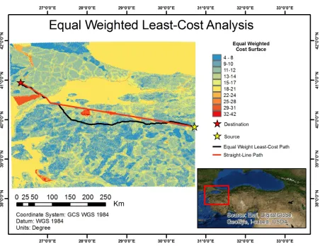
generated a continuous cost surface across the study area that is displayed in Figure 7.

Figure 7. Equal Weight cost surface that was created for the study area. It was from this surface that the least-cost path was derived.

The least-cost path derived from this cost surface is displayed in Figure 8 with its main

25

Figure 8. Least-cost route and straight-line path that was created for cost surface Equal Weights.

Table 1. Least-Cost Path and Straight-Line Path lengths in km and relative cost values using the Equal Weighted Cost Surface. GCS: WGS-84, Projection: Lambert Conformal Conic.

Route Length (km) Relative Cost

Percent Effective

(LC Path/SL Path)

Least-Cost Path 441.00 4084

+37.93%

Straight-Line Path 392.24 6580

The relative cost associated with the path cannot be used as a definite quantitative

meas-urement of the cost of the pipeline but instead is a relative indicator of the risks associated with

straight-line path cost that would be accumulated across the cost surface from the starting

loca-tion to the destinaloca-tion, one can determine the percentage of relative risk that is avoided by the

least-cost route and essentially the effectiveness of the least-cost route.

Table 1 displays the relative costs that are associated with each route and also the percent

effectiveness that the least-cost path obtains when compared to the straight-line path across the

same cost surface. The least-cost path is almost 50 km longer than the straight-line path but is

2500 units less in relative cost indicating that the least-cost path is 38% more effective.

In Figure 8 the highest risk areas that are displayed in red correspond to lakes and

envi-ronmental preserves that are located within the study region. These regions are assigned higher

risk values in the cost surface than other water bodies due to the fact that they are ‘doubly’ risky.

These areas are represented as high risk for multiple criteria, environmental areas and being a

water body. This is why they are of higher cost than the larger water bodies in the study region.

4.2 Weighted Overlay

Multiple cost surfaces were created using the Weighted Overlay tool in the ArcMap

software that designated specific weights to each criterion. Table 2 below displays the weight

amounts for each of the weighted cost surfaces that were created. Each Weighted Overlay

sur-face that was created highlighted a specific criterion or criteria more than others to detail the

im-pact that they had on the least-cost path.

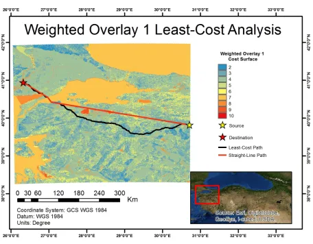
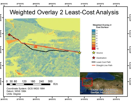
Table 2. Weight Percentages for each criterion in all 3 Weighted Overlay Cost Surfaces.

Cost Surface Criterion Weight Percentage

Weighted Overlay 1

Slope 45%

27

Population 15%

Environmental Areas 10%

Faults 10%

Weighted Overlay 2

Slope 25%

Geology 15%

Population 30%

Environmental Areas 20%

Faults 10%

Weighted Overlay 3

Slope 20%

Geology 35%

Population 10%

Environmental Areas 15%

Faults 20%

The figures below (Figure 9, Figure 10, and Figure 11) display the selected routes for

each of the weighted overlay cost surfaces. The lengths and the associated relative cost for each

29

Figure 11. Least-cost route and straight-line path that was created for cost surface Weighted Overlay 3.

Table 3. Least-Cost Paths and Straight-Line Paths for each of the specified Weighted Overlay Cost Surfaces. Detailed lengths in km and relative cost values for each path on the respected cost surface. GCS: WGS-84, Projection: Lambert Conformal Conic.

Route Cost Surface Length (km) Relative Cost

Percent

Effec-tive

(LC Path/SL

Path)

Least-Cost Path

Weighted

Over-lay 1

448.000 1349

+36.07%

31

Path lay 1

Least-Cost Path

Weighted

Over-lay 2

427.343 1848

+23.83% Straight-Line

Path

Weighted

Over-lay 2

392.238 2426

Least-Cost Path

Weighted

Over-lay 3

460.391 1532

+38.96% Straight-Line

Path

Weighted

Over-lay 3

392.238 2510

The costs for the straight-line paths through each of these cost surfaces are higher than

the costs for the least-cost paths, although the lengths of the least-cost paths are longer. By

exam-ining each Weighted Overlay surface one can see that the highest percent effectiveness was

cal-culated from the third weighted overlay surface with its value of 38.96%. The third weighted

overlay surface placed emphasis on the geological hazards within the area more so than any of

the other criteria. This indicated that the major criteria for the routing in this study region were

the geological hazards that are present.

4.3 TANAP Proposed Route

The main proposed route of TANAP was sourced from the Environmental Assessment

Application that was compiled by Cindar Engineering and Consulting Inc. (“Environmental

In-dependent Assessment Application” 2013). The 2749 GPS points that make up the entire

pipe-line length from the Turkish-Georgian border westwards to the border with Greece, which

gas to Central Europe, is documented within this assessment (“Environmental Independent

As-sessment Application” 2013). The proposed route is displayed in Figure 12 alongside the

multi-ple least cost routes that were created and with Table 4 detailing specific properties of the

pro-posed path.

Figure 12. Displays the least-cost routes derived from all 4 cost surfaces and the proposed TANAP route that was referenced from Cindar Engineering and Consulting Inc. 2013.

Table 4. Detailed length in km and relative cost for proposed TANAP route through each separate cost sur-face. Does not include connection from Canakkale to Tekirdag-Bulgarian border. GCS: WGS-84, Projection: Lambert Conformal Conic.

Route Cost Surface Length (km) Relative Cost

33

Route from TANAP

EIA Report

Weighted Overlay 1 470.615 2429

Weighted Overlay 2 470.615 2999

Weighted Overlay 3 470.615 3053

Table 5. Error polygon areas between each created route and the proposed TANAP route. Area is calculated between two linear features.

Error Polygon Area (km2)

Equal Weighted vs. TANAP 5644

Weighted Overlay 1 vs. TANAP 3311

Weighted Overlay 2 vs. TANAP 4871

Weighted Overlay 3 vs. TANAP 4142

The detailed length and relative cost quantities were compiled using the ESRI ArcMap

10.1 software with the detailed geographic coordinate system and projection listed in the table

above. The costs of the proposed path were extracted from all four different cost surfaces that

were created and excluded the 167 km section that travels north from Çanakkale to Tekirdag and

the Bulgarian-Turkish border. When examining Table 4 the relative costs that were calculated for

the proposed TANAP route from each of the four cost surfaces detail the costs that would be

as-sociated with that route for each surface. These costs were then compared to the least-cost path

5 DISCUSSION

5.1 Trans-Anatolian Natural Gas Pipeline Least-Cost Analysis

When examining the results that were generated from the four cost surfaces within the

study it is clearly evident that the least-cost routing tool is more efficient than a typical

straight-line path. Beginning with the Equal Weighted cost surface, the least-cost route that was

deter-mined detailed a relative cost that was around 38% lower than the straight-line path. The

straight-line path was used as a comparison in that the shortest distance between two points is a

straight-line and would in theory traverse the fewest amount of cells within the cost surface. This

in effect would be assumed to generate the lowest cost through the study area. This is not the

case though due to the specific criteria that were combined together to form the cost surface.

This is where the logic of the least-cost algorithm that is coded within the ArcGIS tool displays

its worth in navigating the highest cost cells while traversing the cost surface from source to

des-tination.

These costs that are accumulated for each derived path are not quantitative figures that

can be used in projects such as engineering designs as these values only display the relative cost

that is associated from traversing the specific cost surface. This relative cost can be compared to

one another in a ratio as shown in Tables 1 and 3 to determine the effectiveness of the least-cost

path but the actual values cannot be listed as official quantitative statistics for the route of the

pipeline. It is also relevant to note that the relative cost values that were calculated for the

Equal-Weighted cost surface cannot be compared directly to the values that were calculated for the

Weighted Overlay cost surfaces due to the different scaling of cost values between the two types

of cost surfaces (Equal Weighted and Weighted Overlay). For this reason also the ratio of

35

When the effectiveness of each route was compared to one another the higher the

effec-tiveness of the route, the better the route was at crossing that specific cost surface. As displayed

in Table 3 the least-cost path that was created across Weighted Overlay 3 was the most efficient

route when compared to the straight-line route. This cost surface focused mainly on highlighting

the geologic hazards that would effect the routing of the pipeline. These geologic hazards were

characterized by the age and lithology present at each location. These ages and lithologic

de-scriptions wee derived from the AGI dataset and provided general dede-scriptions of the surficial

rocks at that geographic location. Younger rocks that were essentially basin infill as the final

tectonic plates converged together to form the Anatolian peninsula were determined to be of

higher risk than older more consolidated rocks in the area (A. Okay 2008; A. I. Okay et al. 2012;

Tamer Y. Duman et al. 2005). These younger basin infill rocks were composed of mainly flysch

and alluvium that was derived from the weathering of the converging volcanic island arcs. The

ages of these geologically young rocks were from mainly Cenozoic to Late Mesozoic and

con-sisted of these flysches and marine sedimentary sequences. These specific lithologies are not able

to withstand very much strain and thus are very prone to fail (T. Y. Duman et al. 2005; Tamer Y.

Duman et al. 2005). Older rocks within this region mainly consist of igneous intrusives and

mé-langes of Precambrian to Late Paleozoic age that were created from the compaction of

accretionary wedges. These consolidated and extremely compacted lithologies are able to

with-stand more strain due to the physical structure of the rocks and are thus less likely to fail (A. I.

Okay et al. 2012; A. Okay 2008; Krushensky 1980). These more structurally sound rocks are less

prone to landslides which are a key hazard in pipeline construction. These pipelines are designed

to last 30-40 years and thus the geologic characteristics as well as the terrain are key elements in

second most important to the geology. These criteria are intricately linked together in the

occur-rence and spatial extent of landslides.

At the beginning of the study the main assumptions of pipeline routing was that

land-slides and terrain hazards would be the most controlling factor in the selection of a viable route

through the study area. The terrain dictates much more so in where the pipeline can be placed

than other criteria such as population. Large diameter pipelines like TANAP can be placed

through urbanized areas if needed but they are not able to traverse very steep gradients composed

of brittle rock. It is due to these reasons and more that the results are not surprising that the

Weighted Overlay 3 cost surface and least-cost route were the most efficient. When comparing

the proposed route, which was highlighted in Appendix 5 of the Environmental Independent

As-sessment (published March 2013), to the least-cost route through Weighted Overlay 3 they are

very similar (See Figure 12). This clearly indicates that certain criteria are much more important

than others in the selection process of where to construct these large diameter pipeline projects.

However when comparing the relative costs between the proposed TANAP route and the

weighted overlay routes the Weighted Overlay 1 route was the most efficient and had the

small-est error area from the proposed route. This error was calculated from the area between the two

linear routes with the smallest area inferring the least error between routes. This weighted

over-lay also had a heavy bias in the slope and lithology of the study area. The teams of engineers at

Cindar Environmental and Consulting Inc that calculated the proposed TANAP route

document-ed in their investigations when the investigation area in their assessments had to be expanddocument-ed in

order to fully investigate the geological and geomorphologic structures that were present

(“Envi-ronmental Independent Assessment Application” 2013). This process also indicates how

37

The fact that the heavy population bias of Weighted Overlay 2 did not result in the

high-est efficiency was a surprise to the assumptions that were compiled at the beginning of this

study. One would think that the highest population density areas would be a major controlling

factor in the site selection of where large-scale projects like TANAP would be routed due to the

influence that citizens would have on construction sites traversing their private land. While this

factor is obviously prominent in the routing process it does seem to take a secondary role to the

other criteria, mainly the geologic and terrain, due to the fact that it is not as definitively fixed as

the other criteria. Land can be acquired and houses moved in part to allow the pipeline to

trav-erse a more suitable gradient of terrain whereas a mountain or steep cliff valley cannot be as

easily remedied. In this sense the construction firm can manipulate this criterion in order to best

suit their needs when constructing the pipeline, whereas the natural landscape and terrain pose a

much more rigid set of criteria.

A key observation to take into account when examining the results from the proposed

TANAP route and the least-cost routes that were experimentally created was that even though

these experimental routes only took into account a very select few criteria they almost mimicked

the proposed route. In Figure 12 one can see that the experimental routes were not sourced from

the exact location where the proposed route entered the study area. This is due to the

ever-changing circumstances when routing large projects such as this pipeline. Cindar Engineering

and Consulting Inc. released these proposed route points after the experimental routes had been

calculated from the listed geographic location from TANAP. Although the source locations for

each route were different, this did not affect the experimental routes significantly enough to

doc-ument. This in turn meant that the other criteria that Cindar Engineering used were responsible

Engineering used many more criteria in their routing process such as: land cover, archaeological

sites, ground conditions, transport access, etc (“Environmental Independent Assessment

Applica-tion” 2013). Although these criteria have their own specific importance the fact that the five

ma-jor criteria that were used provided very similar routes leads one to believe that the processes

used in this thesis could be more efficient. When examining the small-scale restrictions to the

pipeline route all of these minor criteria may come into play more so but for large-scale siting

purposes only major physical criteria need be applied. From this strategy engineers could then

hone the route model in to fit their needs and save time and money in the process by having a

general route plan already calculated.

5.2 Limitations of this Route Model

While this thesis provides a case study on what to consider and how to efficiently create a

least-cost route for a major pipeline project, there are some limitations that are to be considered.

Firstly the scale of the study limits it ability to be very precise about the specific route to

con-struct this pipeline. The study area consists of more than 150,000 square kilometers and the

reso-lution of the data that was used was 90-meter cells. This cell size is very coarse for specific,

de-tailed engineering work that is mandated for a project of this cost and size. Therefore in order to

obtain a more specific and detailed least-cost route, along with a more site specific cost surface,

many small-scale experiments at the proposed sites in Turkey must be performed. This type of

multiple siting investigations was done in the Environmental Independent Assessment, which is

why that assessment was used to display the proposed TANAP route and used as a control to

compare the results of this thesis. Due to timing and the funds of this study I was unable to travel

to the field to collect these measurements. This in part was why the created least-cost paths were

inde-39

pendent assessment right of way width of only 50 meters (“Environmental Independent

Assess-ment Application” 2013). If I had been able to travel to the actual study region and assess the

proposed pipeline corridor more accurately defined specific areas of higher risk would have been

compiled.

Another key limitation of this study was the acquisition of accurate and precise data for

the study area. The area of Western Turkey is not as extensively studied as most parts of the

world therefore it was very difficult to acquire very precise GIS data to implement into the

anal-ysis. One key dataset that was used extensively in the environmental assessment by Cindar

Engi-neering Inc but not within this study was the land use classification for the study area. Land use

classification identifies what the current use of a specific geographic location is and helps with

the routing of this large scale project by helping the planners to find areas of land use that are not

extensively developed. These land use classifications can be determined from remotely sensed

data from satellites such as the Landsat program. In order to make sure that your classifications

are indeed correct from these remotely sensed images you would then need to actually obtain

verification of the land use by either going out to the specific locations or obtain verification

from another person who is there. In this study I was unable to ground-truth any classifications

that I would have interpreted due to the unavailability to travel to these locations firsthand. This

land use dataset would have greatly increased the accuracy and relevance of the least-cost path

analysis by implementing the current use of the land into the created cost surfaces. This extra

criterion would have allowed the least-cost paths to take into account types of land that are most

suitable for construction and therefore less risky.

The lack of precision in other datasets that were used such as population density and fault

did not allow for the most precise results on where the least-cost path should be routed. Similar

datasets in locations such as the United States allow for more detail to be implemented into the

analysis due to the level of detail that is compiled within the datasets. This level of detail only

comes from the amount of previous studies that have taken place within a study area. The

Gen-eral Directorate of MinGen-eral Research and Exploration of Turkey (MTA) provided some GIS data

for the region but overall this data was not very precise. This lack of precision within the datasets

was a key factor in the least-cost analysis and limited the accuracy of the study to only a regional

scale and not site specific.

6 CONCLUSION

The created least-cost paths from this thesis provides the least hazardous pipeline routes

by using the available data that covers the region of Western Turkey. When comparing the

creat-ed routes to the proposcreat-ed TANAP pipeline route that was recently releascreat-ed to the public in

March 2013, the least-cost paths accurately detail routes that are strikingly similar and effective

in providing a path from the documented source and destination points within Western Turkey.

This thesis, using similar studies as background and for reference, combined the key factors in

routing a large-scale pipeline project into a relevant cost surface that was then able to perform a

least-cost path analysis and deliver a connected route. While the thesis had some limitations with

the amount of data available and its precision, the overall result was a viable least-cost path that

satisfied the main regulations with routing this type of infrastructure.

With more precise and higher resolution data the limitations of this study may be

en-41

hance the quality of this model and in turn help to route the Trans-Anatolian Natural Gas

Pipe-line in the least hazardous areas and deliver another stable supply of natural gas to the European

REFERENCES

Aissi, Hassene, Salem Chakhar, and Vincent Mousseau. 2012. “GIS-based Multicriteria

Evaluation Approach for Corridor Siting.” Environment and Planning B-Planning & Design 39

(2): 287–307. doi:10.1068/b37085.

Atkinson, David M., Peter Deadman, Douglas Dudycha, and Stephen Traynor. 2005.

“Multi-criteria Evaluation and Least Cost Path Analysis for an Arctic All-weather Road.”

Ap-plied Geography 25 (4): 287–307. doi:10.1016/j.apgeog.2005.08.001.

Baev, Pavel K., and Indra Øverland. 2010. “The South Stream Versus Nabucco Pipeline

Race: Geopolitical and Economic (ir)rationales and Political Stakes in Mega-projects.”

Interna-tional Affairs 86 (5): 1075–90. doi:10.1111/j.1468-2346.2010.00929.x.

Bagli, Stefano, Davide Geneletti, and Francesco Orsi. 2011. “Routeing of Power Lines

Through Least-cost Path Analysis and Multicriteria Evaluation to Minimise Environmental

Im-pacts.” Environmental Impact Assessment Review 31 (3): 234–39.

doi:10.1016/j.eiar.2010.10.003.

Bolat, Pelin, and Jin Yongxing. 2013. “Risk Assessment of Potential Catastrophic

Acci-dents for Transportation of Special Nuclear Materials Through Turkish Straits.” Energy Policy

56 (May): 126–35. doi:10.1016/j.enpol.2012.12.010.

BP Exploration Ltd. 2013. “Shah Deniz 2 and the Opening of the Southern Corridor”.

Brochure. Baku, Azerbaijan: BP Exploration Shah Deniz Ltd.

http://www.bp.com/content/dam/bp/pdf/Press/shah_deniz_2_brochure_english.pdf.

Brody, Thomas M., Paisly Di Bianca, and Jan Krysa. 2012. “Analysis of Inland Crude

Oil Spill Threats, Vulnerabilities, and Emergency Response in the Midwest United States.” Risk