www.hydrol-earth-syst-sci.net/15/3495/2011/ doi:10.5194/hess-15-3495-2011
© Author(s) 2011. CC Attribution 3.0 License.
Earth System
Sciences
Sand box experiments to evaluate the influence of subsurface
temperature probe design on temperature based water flux
calculation
M. Munz1,2, S. E. Oswald1, and C. Schmidt2
1Institute of Earth and Environmental Science, University of Potsdam, 14476 Potsdam, Germany
2Department of Hydrogeology, Helmholtz Centre for Environmental Research – UFZ, 04318 Leipzig, Germany
Received: 27 May 2011 – Published in Hydrol. Earth Syst. Sci. Discuss.: 24 June 2011 Revised: 27 October 2011 – Accepted: 4 November 2011 – Published: 18 November 2011
Abstract. Quantification of subsurface water fluxes based on the one dimensional solution to the heat transport equa-tion depends on the accuracy of measured subsurface tem-peratures. The influence of temperature probe setup on the accuracy of vertical water flux calculation was systematically evaluated in this experimental study. Four temperature probe setups were installed into a sand box experiment to measure temporal highly resolved vertical temperature profiles under controlled water fluxes in the range of±1.3 m d−1. Pass band
filtering provided amplitude differences and phase shifts of the diurnal temperature signal varying with depth depending on water flux. Amplitude ratios of setups directly installed into the saturated sediment significantly varied with sand box hydraulic gradients. Amplitude ratios provided an accurate basis for the analytical calculation of water flow velocities, which matched measured flow velocities. Calculated flow velocities were sensitive to thermal properties of saturated sediment and to temperature sensor spacing, but insensitive to thermal dispersivity equal to solute dispersivity. Ampli-tude ratios of temperature probe setups indirectly installed into piezometer pipes were influenced by thermal exchange processes within the pipes and significantly varied with wa-ter flux direction only. Temperature time lags of small sensor distances of all setups were found to be insensitive to vertical water flux.
Correspondence to: M. Munz ([email protected])
1 Introduction
Hatch et al., 2006; Rau et al., 2010). Time series methods that determine streambed flux, are based on the quantifica-tion of changes in amplitude (amplitude ratio) and phase shift (time lag) between pairs of subsurface temperature time se-ries. Amplitude and phase information of temperature time series can be derived by pass band filtering (Hatch et al., 2006) or dynamic harmonic regression (Keery et al., 2007) signal processing techniques, both, enabling fast data pro-cessing and fast analytical evaluation. Lautz (2010) tested impacts on analytical flux estimates for the case of violated boundary conditions using numerical simulation. She found the greatest source of error to be due to non-vertical flow in the streambed. Schornberg et al. (2010) assessed the error introduced to the analytical solution provided by Bredehoeft and Papadopolus (1965), which is for the assumption of a heterogenous saturated sediment showing a pronounced con-trast between hydraulic conductivities. The results of their simulations indicate that the method fails to provide reliable discharge estimates. Rau et al. (2010) evaluated measured temperature time series of three Australian rivers using two different analytical solutions and demonstrated inconsisten-cies in flux results between both methods. Jensen and Enges-gaard (2011) compared Darcian flow velocities derived by time series analysis with seepage meter measurements at the Holtum Stream (Denmark) and found noticeable differences in mean flux values and ranges. Applying heat as a tracer is not only limited by inaccuracies of data evaluation, but also by practical limitations such as the accurate measurement of subsurface temperatures.
This experimental study systematically compares the in-fluence of temperature probe setup on amplitude ratio and time lag, and on the overall accuracy of the analytical wa-ter flux calculation of several direct and indirect temperature probe installations. The objectives are to evaluate the poten-tial of temperature amplitude ratio and time lag to be used as targets for analytical flux calculation over a wide range of up-ward and downup-ward fluxes; to show differences between am-plitude ratios and time lags of common and new developed direct and indirect temperature probe setups; and to asses the overall accuracy of the flux calculation depending on tem-perature probe setup. Therefore, temtem-perature time series of a long term sand box experiment were measured at mul-tiple depths under controlled flux conditions ranging from −1.30 m d−1(downward) to 1.29 m d−1(upward). Tempera-ture probes were directly installed into the sediment by lost cone drilling, using a newly developed Multi Level Temper-ature Stick (MLTS) and, indirectly, inserting the tempera-ture probes into a bottom screened and a complete screened piezometer pipe. Measured temperatures were analysed us-ing the time series method introduced by Keery et al. (2007).
2 Methods
2.1 Heat transport theory and data analyses
Temperature time series of the surface water contain com-ponents of various frequencies. These comcom-ponents can be classified into cyclic variations caused by solar radiation, and into random variations caused by short term disturbances of the radiative flux by shading of clouds, vegetation or heat in-troduced by precipitation into the system (Sinokrot and Ste-fan, 1993). As the variation of solar radiation has a daily and annual behaviour, there are theoretically two strong si-nusoidal cyclic components in the temperature time series of frequencies, of one cycle per day and one cycle per year (Keery et al., 2007). The naturally introduced surface wa-ter temperature signal propagates into the sediment. Thereby the signal is reduced in amplitude and shifted in time de-pending on the thermal properties of the streambed and ac-tual surface water-groundwater exchange fluxes (Constantz and Stonestrom, 2003; Keery et al., 2007; Hatch et al., 2006; Rau et al., 2010).
Stallman (1965) developed a complete analytical solution that simultaneously describes the heat transport by conduc-tion and heat transport by advecconduc-tion (convecconduc-tion) for steady water flow. For this, he assumed a sinusoidal temperature oscillation of constant amplitude at the surface-subsurface interface and a constant temperature at infinite depth. This approach can be used to determine constant and uniform in-filtration rates or exchange fluxes normal to the surface in a homogeneous medium.
Keery et al. (2007) reformulated this solution to compute an unknown vertical water flux (q, m d−1) with given
ob-servations of oscillating temperatures at two depths below the surface. They derived one implicit formulation based on thermal properties of the system and amplitude attenuations (Eq. 1), and one explicit formulation based on thermal prop-erties of the system and time lags (Eq. 2):
0 = H
3D
4z
!
q3 − 5H
2D2
4z2
!
q2 + 2H D
3 z3
!
q
+ π c ρ
λeτ
2 − D
4
z4 (1)
where
D = ln A
z+1z,t+1t Az,t
and H = cwρw
λe .
Az+1z,t+1t
Az,t is the amplitude ratio of the amplitude of a single
frequency oscillation at depthz+1zand timet+1t and at depthz(m) and timet (s), respectively. τ is the time period (s) of that frequency,ρ is the density of saturated sediment (kg m−3),ρw is the density of water (kg m−3),cis the
spe-cific heat capacity of the saturated sediment (J kg−1K−1),cw
the effective thermal conductivity of the saturated sediment (W m−1K−1).
The explicit formulation based on time lags is:
q = c
2ρ2z2 1t2c2
wρw2
− 16π
21t2λ2 e τ2z2c2
wρw2
!12
(2) where1tis the time lag between time of amplitude atz+1z
and time of amplitude atz,1z is the vertical distance be-tween two vertical measurement points. The resulting flux of Eq. (1) is positive in downward and negative in upward di-rection, while Eq. (2) does not allow distinguishing between flux directions.
To satisfy the upper boundary condition of the analytical solution, the most pronounced temperature frequency of one cycle per day was isolated of the temperature time series by a pass band filter with a Kaiser window. The filter was set to a pass band frequency range of 0.9 d−1to 1.1 d−1and to stop band frequencies of<0.6 d−1and>1.4 d−1as suggested by Hatch et al. (2006). To avoid edge effects, the first and the last seven days of data were used to extent the measured tem-perature time series. Finally, a peak detection routine was applied to the filtered time series to detect daily maxima (am-plitude) and their exact timing. The results were plotted and checked visually for completeness of corresponding peaks. Daily amplitudes and timings were used to calculate ampli-tude ratios and phase shifts, which were used to calculate ver-tical sand box water flow velocities based on Eqs. (1) and (2). To compare the amplitude ratios and time lags for each hy-draulic head difference (1h), the non-parametric measures median and 95 % confidence interval of the median were used. It was visually checked whether or not the 95 % con-fidence intervals of each median overlap. In case they do not overlap, the amplitude ratios and the time lags occur-ring for each1hare seen as significantly different from each other at the 5 % significance level and are regarded to be sensitive to water flux. Based on this amplitude ratio and time lag sensitivity to different magnitudes of water flux, we evaluated whether subsurface temperature patterns provide a sufficient basis for analytical, temperature-based water flux calculations.
To characterize experimental water fluxes in terms of dom-inant heat transport mechanism and thermal stability the di-mensionless Peclet and Rayleigh number of energy transport have been applied. The Peclet number is the ratio of energy transported by advection to the energy transported by con-duction (Domenico and Schwartz, 1990). Peclet numbers greater than one indicate that advective heat transport domi-nates over conductive heat transport. The Rayleigh number is the ratio of energy transported by free convection to the energy transported by conduction (Domenico and Schwartz, 1990). Free convection occurs when fluid flow is forced by buoyancy due to density differences where a dense fluid over-lies a less dense one; caused by temperature or solute concen-tration gradients.
2.2 Experimental setup
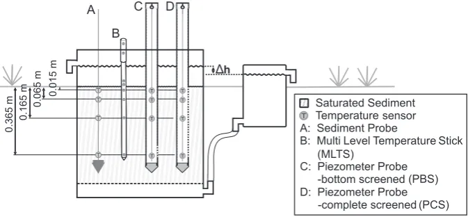
The model apparatus consists of a polyvinylchloride barrel with a diameter of 0.68 m and a total height of 0.80 m. To create barrel in and outlets two 34 inch (1.91 cm) openings were drilled at 0.04 m and 0.7 m above the bottom. At 0.08 m above the bottom in/outlet a stainless steel frame covered with stainless steel gauze was exactly fitted in the barrel and sealed with silicon on its sides. Above that frame, the barrel was filled with a 0.5 m thick homogeneous, medium-grained quartz sand layer. The dry sand was slowly trickled into the barrel and was stirred from time to time to assure a homo-geneous sediment distribution as good as possible. The bar-rel was buried into the ground to the height of the sediment surface at a sun-exposed position at an experimental field site at the Helmholtz Centre for Environmental Research – UFZ in the city of Leipzig, Germany (Fig. 1). Consequently, the buried part of the barrel was in thermal contact with the natural ground sediment and thus with the natural thermal regime. The non-buried part was in thermal contact with the atmosphere.
A conventional 10 l bucket, with two34inch openings built in, one below the top and one above the bottom of the bucket, was used as vertically adjustable water reservoir to control the vertical hydraulic gradient. The bucket’s bottom opening and the barrel’s bottom in/outlet were connected via a 34inch ordinary garden tube. The barrel sediment was slowly satu-rated with water supplied through the barrel bottom inlet. In total 58 l were necessary to saturate the sediment.
Vertical water fluxes were generated by adjusting the abso-lute height of the bucket to create hydraulic head differences (1h) from −0.026 m to 0.026 m in 8 steps. Negative gra-dients, i.e. the water level of the barrel was higher than the water level of the bucket, generated vertical downward flux through the sediment. Therefore water was introduced into the top of the barrel, filtrated through the sediment and left the system through the upper bucket opening. The water sup-ply was adjusted to enable a minor water volume discharge through the barrel top outlet avoiding large water level fluc-tuations. In contrast, positive gradients, i.e. the water level of the barrel was lower than the water level of the bucket, generated vertical upward flux. Upward fluxes were induced by introducing water into the top of the bucket which flowed through the sediment body and left the system through the barrel top outlet. Again the water supply was adjusted in a way to enable water discharge through the upper bucket opening avoiding large water level and temperature fluctua-tions within the bucket. The bucket was covered to prevent rain entering into the system.
(MLTS)
(PBS)
[image:4.595.130.467.63.219.2](PCS) sensor
Fig. 1. Experimental setup of sand box experiment and of temperature probe installations(A–D)with temperature sensors at four different depths (0.015 m–0.365 m) below ground surface.
figure
35
Fig. 1. Experimental setup of sand box experiment and of temperature probe installations (A)–(D) with temperature sensors at four different depths (0.015 m–0.365 m) below ground surface.
constant hydraulic gradients were averaged to the gradient dependent flux (q). The 95 % confidence intervals ofqwere calculated and used to test whether the fluxes were signifi-cantly different between the different hydraulic gradients. 2.3 Temperature probe installation
The sand box was instrumented at a depth of 0.015 m, 0.065 m, 0.165 m and 0.365 m below the sediment surface with temperature sensors using the setups described in the following. Preliminary calculations using Keery’s analyti-cal solution (Eq. 1) in the forward analyti-calculation mode were conducted to define appropriate sensor depths according to the given hydraulic head gradients and expected atmospheric temperature variations. The sensors were placed to capture dampening and time lag in temperature signal for high up-ward fluxes (0.065 m), at the depth of 0.165 m at which daily temperature variations are damped 63 % for the purely con-ductive case (Dampening depth, cp. Stonestrom and Blasch, 2003) and at 0.365 m to ensure sufficient dampening and time lag for high downward fluxes. The Minimum instal-lation depth of 0.015 m was limited by the Sediment Probe setup that the uppermost sensor was slightly covered by the sediment.
1. Vertical installation of TidbiTs within the sediment (Sediment Probe): the TidbiT v2 temperature sensor (Onset computer cooperation, Pocasset, Massachusetts, USA) contains a thermistor integrated with signal-conditioning circuitry, a real time clock and a mem-ory unit. The constituent parts are inserted in a 3 cm×1.7 cm large epoxy case which is waterproof up to 305 m depth. The measurement accuracy is 0.2◦C over a range from 0 to 50◦C. The sensor resolution is 0.02◦C with a response time of 5 min in water.
The TidbiT temperature sensor were connected via a thin fibre at predefined intervals and fixed to a steel cone. The cone was loosely fitted to a steel pipe with an
inside diameter of 0.04 m and a length of 1.50 m. The pipe was driven into the barrel sediment using a sledge hammer. A metal rod was inserted down the pipe and pushed to detach the cone from the metal pipe while the pipe was slowly removed (lost cone drilling). The fibre with the connected TidbiTs was held tight all the time to ensure the sensors being in the right position while the sediment was collapsing. Thus, the temperature sensors are directly in thermal contact with sediment.
2. Installation of the Multi Level Temperature Stick (MLTS): the Multi Level Temperature Stick (Umwelt und Ingenieurtechnik GmbH, Dresden, Germany) is a polyoxymethylene stick (total length of 0.657 m and a diameter of 0.02 m) with eight integrated TSIC-506 temperature sensors (sensor depth could be individually defined by the user before production). These sensors are based on a semiconductor resistor embedded in an integrated circuit for conservation to a linear electrical output. The thermal contact of the sensors to the sur-rounding material is ensured through thin stainless steel flat blanks. The temperature is measured with each sen-sor simultaneously with an accuracy of 0.07◦C over a
range from 5 to 45◦C. The sensor resolution is 0.04◦C.
The MLTS was pushed into the sediment to a depth of 0.4 m, so that four sensors are in the sediment and two sensors log the surface water temperature.
screen the piezometers the pipes were screwed at three sides with a thin sawing blade (0.05 mm) in regular dis-tances of 5 mm. The distance between drive point and beginning of the screen allows little sediment particles to settle down inside the piezometer without clogging the screen. The TidbiT temperature sensors were con-nected via a thin fibre at predefined intervals. This sen-sor chain was suspended within the piezometer. 4. Vertical installation of TidbiTs inside a complete
screened piezometer (PCS): the installation of the PCS is the same as described for the PBS except the piezometer pipe which was screened 0.06 m above the drive point over a section of 0.36 m, in a total depth from 0.01 to 0.37 m. The complete screen allows barrier free heat propagation between the temperature sensors and the sediment with negligible influence of the piezometer material. Because of the limited number of temperature sensors available, the TidbiT sensor chain (cp. setup 3) was switched between the PBS and PCS after half of the time of equal hydraulic gradient. To check thermal regime of the other pipe respectively, one TidbiT tem-perature sensor was suspended within the piezometer at a depth of 0.165 m (single piezometer sensor).
All sensors were calibrated in the upper water reservoir of the barrel during five days. For these data, correction factors were established by linear regression of each sensor with a reference sensor. All temperature sensors were set to a 15 min measurement interval.
The previously described Sediment Probe and PBS setups were chosen for installation as they are the most common to install temperature sensors within saturated sediment. The Sediment Probe was embedded directly within the sediment. The time to reach the thermal equilibration between the tem-perature sensors and saturated sediment is supposed to be less than the monitoring interval of 15 min. Therefore the Sediment Probe setup was assumed to be the least intrusive setup and that it was in best thermal contact with the satu-rated sediment. The PBS temperature sensors were sepasatu-rated from the saturated sediment by ideally non-moving water and by the piezometer side wall. To potentially reduce the ef-fect of piezometer side wall the PCS setup was designed as a modification of the PBS setup. The MLTS was used as it is a newly developed probe design characterized by good practical application in terms of installation, known accurate sensor spacing and data availability during operation. The MLTS sensors were embedded in a HDPE rod separated by small stainless steel plates from the saturated sediment.
Each profile probe setup, having four temperature sensors recording the sediment temperatures, allows calculation of amplitude ratio and phase shift relations for six sensor pairs. All sensor combinations of all installations were evaluated with respect to the sensitivity of their amplitude ratios and time lags to variations of1h. For brevity only the results
of sensor pairs which cover minimum (pair0.065−0.015),
in-termediate (pair0.165−0.065) and maximum sensor distances
(pair0.365−0.015) are discussed (subscript specifies depth of
installation of used temperature sensors). However, they pro-vide a sufficient overview on the experimental results as all other sensor pairs overlap, i.e. use equal temperature sensors but integrate over different segments of the sand box, and are therefore potentially redundant.
2.4 Estimation of saturated sediment thermal properties and sensitivity analysis
To calculate vertical flow velocities based on Eqs. (1) and (2), thermal properties of the saturated sediment need to be de-termined. As these values are difficult to measure outside the laboratory (Stonestrom and Blasch, 2003), we used liter-ature based values. Heat capacities of porous materials de-pend on their composition and bulk density (Stonestrom and Blasch, 2003). Thus the volumetric heat capacity of the bar-rel sediment was calculated from the volume-weighted sum of density and the volume-weighted sum of heat capacities of constituents making up the saturated sediment based on experimental estimated total porosity. The thermal conduc-tivity of porous materials depends upon the composition and arrangement of the solid phase. Due to the complexities of pore geometry, this dependence is non-linear and difficult to predict (Wierenga et al., 1969). The thermal conductivity of saturated sediment was calculated from the volume-weighted sum of thermal conductivities of constituents making up the saturated sediment.
The literature based thermal properties were improved during calibration. The calibration was restricted to exper-imental data for no flow condition, e.g.δh= 0 and vertical flow velocity = 0 as there will be no uncertainties introduced to the calibration procedure due to uncertainties of experi-mentally measured water flux. As volumetric heat capacity and thermal conductivity are integrated as quotient (recipro-cal of thermal diffusivity in Eq. 1) they are dependent of each other. Therefore the thermal conductivity, as it is seen to be more uncertain in its literature based assumption; was cali-brated exclusively, in order to minimize the root mean square error (RMSE) between observed and calculated vertical wa-ter flux. Calibrated thermal properties were used for all flux calculations.
2.5 Impact of thermal dispersivity on vertical sand box water flow velocities
Since there is an ongoing discussion about the effects of thermal dispersion on vertical flow velocities (Keery et al., 2007; Hatch et al., 2006), we also quantified the sensitivity of flow velocity to thermal dispersion. In our analysis, ther-mal dispersion is treated in analogy to the solute dispersion. The thermal dispersion (Dispth) is the sum of the bulk soil
thermal conductivity with stationary fluids and a kinematic thermal dispersion term, resulting from the heterogeneity of water velocities within and between water-filled sediment pores. To account for the two processes, Dispth is defined
as (Anderson, 2005): Dispth = λe
c ρ =
λ0
c ρ +αth × |q| (3)
whereλeis the effective thermal conductivity of the saturated
sediment (W m−1K−1),λ0is the baseline thermal
conductiv-ity in absence of fluid flow (W m−1K−1) andαthis the
ther-mal dispersivity (m). Some researchers argue that values of thermal dispersion are comparable to those of conservative solute dispersion (de Marsily, 1986; Hopmans et al., 2002) while others conclude that the effect of thermal dispersion (αth× |q|) is negligible compared to the baseline thermal
dif-fusivity (Bear, 1972; Ingebritsen and Sanford, 1998). Thus, to test the sensitivity of calculated flow velocity to thermal dispersion we assumed the thermal dispersivity to be in the range of solute dispersivities observed by the solute tracer experiment.
To solve the 1-D heat transport equation by means of an analytical solution including convective, conductive and dis-persive heat transport, we used the solution presented by Hatch et al. (2006). Their analytical solution is based on the same assumptions and boundary conditions as the Keery et al. (2007) solution. The main difference is that Hatch et al. (2006) defined the effective thermal diffusivity analogous to Eq. (3), while Keery et al. (2007) set the effective thermal diffusivity equal to the baseline thermal diffusivity.
3 Results and discussion 3.1 Experimental flux
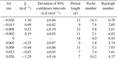
The averaged, gradient-dependent water fluxes in the sand box and their 95 % confidence intervals are given in Ta-ble 1. Ideally one would expect constant discharges as long as 1h is kept constant. However, we observed variations ofq during constant1hwhich were caused by the temper-ature dependency of hydraulic conductivity as well as by disturbances of the experiment during operation. The ef-fect of stream water temperature on hydraulic conductivity and streambed flux in natural systems is shown by Con-stantz et al. (1994) and Storey et al. (2003). The distur-bances mainly occurred at barrel and bucket outlets where
Table 1. Defined hydraulic head differences (1h) of sand box ex-periment, averaged gradient dependent fluxes at system outlet (q) with corresponding deviations of 95 % confidence intervals toq, period length of constant hydraulic gradient and calculated Peclet and Rayleigh numbers of each1hcondition.
1h q Deviation of 95% Period Peclet Rayleigh (m) (m d−1) confidence intervals length number number
toq(m d−1) (d)
−0.026 1.30 ±0.04 12 14.3 0.78
−0.013 0.69 ±0.02 9 7.6 2.05
−0.008 0.53 ±0.10 12 5.8 2.61
−0.002 0.19 ±0.03 11 2.1 6.02
0 – – 18 0.0 6.95
0.002 −0.25 ±0.07 9 2.8 5.74
0.008 −0.48 ±0.06 11 5.3 7.03
0.013 −0.67 ±0.03 7 7.4 3.61
0.026 −1.29 ±0.16 7 14.2 4.37
slugs and polls caused time dependent1hvariations up to 0.002 m; but variations of q during constant 1h condition remained small compared to differences betweenq. Differ-ences between q were significant on the basis of the 95 % confidence interval. The average discharges ranged between −1.30 m d−1 to 1.29 m d−1 (Table 1) and therewith agree well with water fluxes typically observed in natural surface water-groundwater systems (Conant, 2004).
Peclet numbers show that the ratio of convective to con-ductive heat transport varied in dependence of1h(Table 1). Experimental flux conditions were dominated by forced con-vective heat transport also for 1h= 0.002 m indicated by Peclet numbers greater than one. Only for1h= 0 convec-tive heat transport did not occur and the system was driven by pure heat conduction. Rayleigh numbers (Table 1) less than the critical Rayleigh number of 4π2 (Lapwood, 1948; Bear, 1972) indicate that measured temperature gradients were too small to cause substantial instabilities of thermal flow regime. Thus, a 1-D conductive-convective heat trans-port model can accurately describe the experimental thermal regime.
In order to determine hydraulic and hydromechanic sed-iment properties a conservative salt tracer expersed-iment was conducted under a downward flow condition. The tracer was initiated as step pulse injection to the upper barrel water reservoir. Initial concentration at the upper barrel water reservoir was 0.60 g l−1 which was below the
esti-mated threshold concentration for the onset of free convec-tion (0.66 g l−1). The measured discharge and arrival time of maximal tracer concentration were used to calculate the effective porosity (ne) and saturated hydraulic conductivity
(Ksat) based on Darcy’s law. An initial estimate of the
[image:6.595.308.549.141.264.2]Table 2. Sand box characteristics and sediment hydraulic properties.
Parameter Value
Sandbox surface area (A) 0.350 m2
Total porosity (n) 0.370
Effective porosity (ne) 0.330
Saturated hydraulic conductivity (Ksat) 2.24×10⁻⁴m s−1 Dispersion coefficient (DDisp) 1.5×10⁻⁷m2s−1
Longitudinal dispersivity (α) 0.013 m
temporal moments of the tracer break through curves (Cirpka and Kitanidis, 2000, 2001). Calculated sediment properties are presented in Table 2.
3.2 Relations of amplitude ratio and time lag of the sediment probe to hydraulic head differences The Sediment Probe setup was used to analyse the behaviour of amplitude ratios and time lags in relation to specified1h
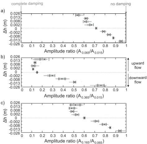
because this setup was assumed to be the least intrusive setup and to be in best thermal contact with the saturated sediment. Figure 2 shows daily amplitude ratio distributions of se-lected sensor pairs depending on1h. The overall range of amplitude ratios was between 0 (completely damped) and 1 (no damping) and illustrates the damping of amplitudes while heat propagates through saturated sediment. Amplitude ra-tios decreased with increasing 1h and increasing sensor spacing (Fig. 2). Thus amplitude ratios were dependent on hydraulic conditions and monitoring depth.
The sensor pair0.065−0.015 showed significant differences
between the amplitude ratios of all 1h with exception of the pair wise comparison of1h= 0.008 m and1h= 0.013 m (Fig. 2a); accurately reflecting differences betweenq.
The deep sensor pair0.365−0.015indicated significant
differ-ences from1h=−0.026 m up to1h= 0.002 m only (Fig. 2b) and the intermediate sensor pair0.165−0.065 indicated
signif-icant differences from 1h=−0.026 m up to 1h= 0.008 m (Fig. 2c). There was a lack of significance during higher upward fluxes. Effects evoked by temperature changes due to heat introduced by rain in the upper water reservoir will be recognized and no additional heat sources occurring in the soil occasionally could be detected. Therefore the most reasonable explanation of this effect was that heat was intro-duced into the system by temperature oscillations within the bucket influencing the deep temperature sensors. As a con-sequence the assumed condition of constant temperature at the bottom of the sandbox was violated. With increasing up-ward fluxes, the effect of variable water temperatures at the bottom inlet became more pronounced. This constrained the validity of analytical solution for1h= 0.013 m and 0.026 m when sensor pairs with deep temperature sensors were used.
0 0.1 0.2 0.3 0.4 0.5 0.6 0.7 0.8 0.9 1
-0.026 -0.013 -0.008
-0.0020
0.002 0.008 0.013 0.026
Δ
h (m)
Amplitude ratio (A. . 0.065/A0.015)
-0.026 -0.013 -0.008
-0.0020
0.002 0.008 0.013 0.026
Δ
h (m)
Amplitude ratio (A. . 0.365/A0.015)
-0.026 -0.013 -0.008
-0.0020
0.002 0.008 0.013 0.026
Δ
h (m)
Amplitude ratio (A0.165/A0.065) a)
b)
c)
0 0.1 0.2 0.3 0.4 0.5 0.6 0.7 0.8 0.9 1
upward flow downward
flow
0 0.1 0.2 0.3 0.4 0.5 0.6 0.7 0.8 0.9 1
[image:7.595.51.284.98.190.2]no damping complete damping
Fig. 2. Daily amplitude ratio distribution of Sediment Probe – sen-sor pairs 0.065–0.015 (a), 0.365–0.015 (b) and 0.165–0.065 (c) of all sand box hydraulic head differences. Data distribution of each condition is shown by box plot (gray shape) with median value of daily amplitude ratios (black dot) and the corresponding 95 % con-fidence intervals of median value (black mark). Note that a negative hydraulic head difference indicates water flux in vertical downward direction.
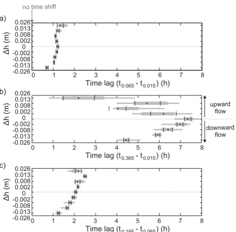
In a similar manner as the temperature time signal was re-duced in amplitude it was also shifted in time. The main difference of time shift compared to amplitude ratio is that it is only dependent on flux magnitudes but independent of the flux direction (Eq. 2). Hence, water fluxes of the same magnitude but different direction will result in identical time lags. The results for sensor pair0.065−0.015 (Fig. 3a)
con-firmed these theoretical relations. Here time lags between
1h=−0.002 and 1h= 0.002 as well as time lags between
1h=−0.008 m and1h= 0.008 m were found to be similar. In contrast, time lags of sensor pair0.365−0.015 (Fig. 3b) and
sensor pair0.165−0.065(Fig. 3c) did not confirm the similarity
of time lags for equal absolute hydraulic head differences. The comparison between time lags of the same flux direc-tion of the shallow sensor pair0.065−0.015shows small, partly
non-significant differences between1hconditions. In con-trast, time lags of the intermediate sensor pair0.165−0.065
dif-fered significantly for all negative1h. Time lags of the deep sensor pair0.365−0.015differed significantly for1hconditions
0 1 2 3 4 5 6 7 8
Time lag (t0.065- t0.015) (h)
Time lag (t0.365- t0.015) (h)
Time lag (t0.165- t0.065) (h)
-0.026 -0.013 -0.008 -0.0020 0.002 0.008 0.013 0.026
Δ
h (m)
-0.026 -0.013 -0.008 -0.0020 0.002 0.008 0.013 0.026
Δ
h (m)
-0.026 -0.013 -0.008 -0.0020 0.002 0.008 0.013 0.026
Δ
h (m)
a)
b)
c)
upward flow
downward flow
0 1 2 3 4 5 6 7 8
0 1 2 3 4 5 6 7 8
[image:8.595.50.286.60.291.2]no time shift
Fig. 3. Daily time lag distribution of Sediment Probe – sensor pairs 0.065–0.015 (a), 0.365–0.015 (b) and 0.165–0.065 (c) of all sand box hydraulic head differences. Data distribution of each condi-tion is shown by box plot (gray shape) with median value of daily amplitude ratios (black dot) and the corresponding 95 % confidence intervals of median value (black mark). Note that a negative hy-draulic head difference indicates water flux in vertical downward direction.
In general, the time lags are less sensitive to1hthan the amplitude ratios. In turn, the time lags will remain suffi-ciently large to resolve high flow velocities up to±10 m d−1 (Hatch et al., 2006). Hatch et al. (2006) developed theoretical type curves for amplitude ratio and phase shift as a function of flow rates for different streambed measurement spacing. Our experimental results are in agreement with the theoreti-cal predictions at least for the tested flow range.
Success of quantifying exchange fluxes based on temper-ature measurements is dependent on the appropriate place-ment of temperature sensors. Decision of placeplace-ment depends on hydraulic and thermal properties of the sediment, sur-face water temperature amplitude and pore water velocities. We used preliminary calculations to realize an appropriate sensor placement for the expected experimental conditions (cp. Sect. 2.3). Furthermore a critical evaluation of bound-ary conditions is essential to apply analytical solutions for vertical flux calculation. Also in natural systems, ground-water temperatures are not necessarily constant, especially in small, upland rivers characterized by shallow aquifers and which are strongly fed by groundwater. For this reason, the sources of subsurface temperature variability need to be con-sidered for the correct interpretation of the obtained ampli-tude ratios and time lags.
All in all, the evaluation of the experimental data revealed that the Sediment Probe setup provided amplitude ratios suf-ficient to resolve sediment water fluxes of −1.30 m d−1 to
1.29 m d−1 when daily amplitudes of 2◦C were present in the surface water. Larger sensor distances would be needed to resolve higher downward fluxes, as otherwise the observed amplitudes may not be sufficiently damped. Only the large temperature sensor distance provided time lags sensitive to experimental fluxes for the given surface water amplitudes. Generally, sensors placed sufficiently close to the sediment surface to be influenced by the diurnal thermal signal had highest accuracy to resolve tested flux magnitudes by the am-plitude ratio method.
3.3 Differences of amplitude ratio and time lag between temperature probe setups
In Sect. 3.2, the differences of amplitude ratios and time lags between 1h conditions of the Sediment Probe setup were analyzed. Based on these findings the general behaviour of amplitude ratios and time lags of Sediment Probe (Fig. 1, setup A) were compared to amplitude ratios and time lags of MLTS (B), PBS (C) and PCS (D), respectively.
Cardenas (2010) showed that the temperature measured inside a pipe buried in the sediment is lagged and damped compared to the temperature outside of the pipe, violating the assumption that monitored temperatures are representative of the saturated sediment. However, he conclude that methods using amplitude ratios and time lags to derive vertical water fluxes are not sensitive to effects of thermal insulation. The effect of thermal insulation would be equal for each sensor of the corresponding setup. Accordingly, these effects would cancel out if quotients or differences of sensors are used for interpretation of measured temperatures.
3.3.1 Sediment Probe vs. MLTS
The comparison of Sediment Probe and MLTS shows that the calculated daily amplitude ratios (RMSE = 0.01◦C) and time lags (RMSE = 0.28 h) were in good agreement for both setups for a wide range of downward flow conditions (Fig. 4a). For upward flow conditions (positive 1h) we observed a slight underestimation of MLTS amplitude ra-tios (RMSE = 0.03◦C) and a more obvious overestimation of
MLTS time lags (RMSE = 0.45 h).
For downward flow conditions heat transport is dominated by advection. The thermal exchange between the fluid and MLTS was practically equal to thermal exchange between fluid and Sediment Probe yielding to comparable amplitude ratios and time lags. For upward flow conditions the direction of advection is directly opposed to heat conduction into the sediment.
a) b) c)
f) e)
d)
Ar ML
TS
Ar Sediment Probe
Ar PBS Ar PCS
Ar Sediment Probe Ar Sediment Probe
Δt
ML
TS (h)
Δt PBS
(h)
Δt PCS
(h)
[image:9.595.130.465.64.297.2]Δt Sediment Probe(h) Δt Sediment Probe (h) Δt Sediment Probe (h)
Fig. 4. Scatter plots of amplitude ratio of Sediment Probe vs. amplitude ratio of Multi Level Temperature Stick-MLTS (a), bottom screened Piezometer Probe-PBS (b) and complete screened Piezometer Probe-PCS (c) and scatter plots of time lag of Sediment Probe vs. time lag of MLTS (d), PBS (e) and PCS (f) of all daily ratios of sensor pairs 0.065–0.015, 0.365–0.015 and 0.165–0.065. The diagonal line is the 1:1 line.
and MLTS. The main material of MLTS is HDPE which is characterized by a higher volumetric heat capacity and lower heat conductivity than the quartz sand (Table 3). With higher volumetric heat capacity more energy is absorbed by the same material volume. Differences in heat capacities caused an increased damping of temperatures for MLTS compared to the true temperature signal occurring within the saturated sediment. The resulting MLTS amplitude ratios were lower than the Sediment Probe amplitude ratios (Fig. 4a).
Lower thermal conductivity caused an increased phase shift, e.g. the deep sensors of MLTS reached their peak tem-perature later than true temtem-perature signal occurring within the saturated sediment. Thus differences in thermal conduc-tivity caused higher time lags of MLTS than of Sediment Probe (Fig. 4d). The deviations of the time lags between Sed-iment Probe and MLTS setup were more pronounced than the deviations of amplitude ratios. This is because the thermal conductivity of HDPE is more than one order of magnitude lower than thermal conductivity of quartz whereby the heat capacity of HDPE is within the same order of magnitude as the heat capacity of quartz (Table 3).
Differences between Sediment Probe and MLTS only oc-curred when heat conduction became the dominant process of downward directed heat transport. Thereby deviations be-tween temperature probe setups increased with depth of tem-perature probe installation, e.g. lowest deviations between amplitude ratios and time lags occurred for sensor pairs lo-cated close to the surface. As the volumetric heat capacity of HDPE is only 11 % higher than the volumetric heat capacity
of quartz sediment deviations in amplitude ratios between Sediment Probe and MLTS remained small, especially for sensor pair0.065−0.015 and pair0.165−0.065. Thus, MLTS
am-plitude ratios of sensor pair0.065−0.015and pair0.165−0.065can
be used for appropriate estimation of vertical flow velocities. The MLTS setup is suitable to calculate water fluxes of at least−1.30 m d−1to 1.29 m d−1providing that the
tempera-ture sensors are installed in the thermally active zone of the saturated sediment (e.g. sensor pair0.065−0.015). In contrast,
the calculation of flow velocities using MLTS time lags was uncertain due to the general insensitivity of time lags to small flow velocities. As the magnitude of deviation between Sed-iment Probe and MLTS time lags was dependent on temper-ature sensor distance it was not possible to establish a simple conversion factor to compensate setup dependent differences between Sediment Probe and MLTS.
The general differences of MLTS derived amplitude ratios for all1hwere comparable to the characteristics of Sediment Probe amplitude ratios. Also the MLTS setup could be used to significantly differ between1hconditions from−0.026 m to 0.026 m as long as temperature sensors installed within the sediment cover small distances of 0.05 m and high distances of 0.35 m.
3.3.2 Sediment probe vs. PBS
Table 3. Thermal properties of sand box individual phases -water, quartz and HDPE- and of saturated porous media.
Density Heat capacity Vol. Heat capacity Conductivity Diffusivity
(ρw, (c, (cvol, (λe, (λcρe,
kg m−3) J kg−1K−1) J m−3K−1) W m−1K−1) m2s−1)
Water 1000a 4182a 4 182 000 0.60a 1.43×10⁻⁷
Quartz 2700b 733b 1 900 000 8.40b 4.20×10⁻⁶
Saturated sediment 2140 1870 4 000 000 5.44 2.69×10⁻⁶
Saturated sediment-calibrated – – 4 000 000 4.75 1.19×10⁻⁶
HDPEc – – 2 137 500 0.49 2.42×10⁻⁴
aCarlslaw and Jaeger (1959);bvan Wijk and de Vries (1966);cwww.matbase.com/material/polymers/commodity/hdpe/properties
time lags were shorter (RMSE = 1.1 h) than the correspond-ing Sediment Probe amplitude ratios and time lags. These de-viations were caused by vertical thermal exchange processes occurring within the piezometer pipe independent of the sat-urated sediment thermal regime.
This might be caused by the onset of heat transport by free convection within the piezometer pipe. Maximal daily temperatures within the piezometer pipe vertically de-creased. While shallow sediment temperatures decreased faster than deep sediment temperatures during nightly atmo-spheric cooling, temperatures of different PBS depth equi-librated (Fig. 5). We observed that at the time the temper-atures of different observation depths reached equality, the temperatures started to decrease simultaneously until mini-mum atmospheric temperatures were reached (Fig. 5). Be-cause of these effects minimum temperatures of PBC were nearly identical whereas Sediment Probe temperatures ver-tically increased with increasing depth. Resulting minimum temperatures at shallow PBS sensors (0.015 m and 0.065 m) were higher and temperatures at deep PBS sensors (0.165 m and 0.365 m) were lower than temperatures occurring within the saturated sediment (Fig. 5). In consequence tempera-ture amplitudes at depth of 0.015 m and 0.065 m were lower and temperature amplitudes at depth of 0.165 m and 0.365 m were higher than corresponding sediment temperature ampli-tudes causing the general overestimation of Sediment Probe vs. PBS amplitude ratios (Fig. 4b).
Also the large underestimation of PBS time lags was a result of thermal exchange processes within the piezometer pipe. PBS temperature maxima of deep sensors (at 0.165 and 0.365 m) were reached earlier than maximum temperatures occurring within the saturated sediment (Fig. 5) causing lower time lags of PBS (Fig. 4e). We also observed few PBS amplitude ratios that were lower and PBS time lags that were higher than the corresponding Sediment Probe amplitude ra-tios (Fig. 4b) and time lags (Fig. 4e). These deviations oc-curred when vertical thermal exchange processes within the piezometer pipe were absent. Thereby the measured tem-peratures at 0.015 m were constantly higher than measured temperatures at 0.065 m (stable thermal stratification). Such
Sediment Probes Piezometer Probes
0.015 m 0.065 m 0.165 m 0.365 m 28
27 26 25
24 23
22 21 29
T
emperature (°C)
12:00 00:00 11:45
Time
Fig. 5. Measured average daily temperature cycle of the Sedi-ment and bottom screened Piezometer Probe of no flow condition (1h= 0).
conditions were observed during experimental upward flow and low atmospheric temperature variations. For these ex-perimental conditions, differences in heat capacities of PBS and saturated sediment caused an increased damping of PBS temperatures compared to the true temperature signal within the saturated sediment, yielding to lower amplitude ratios of the PBS (Fig. 4b). Higher time lags of PBS compared to Sed-iment Probe (Fig. 4e) were a result of lower thermal conduc-tivity of water than of saturated sediment (Table 3). Thereby the induced temperature signal propagated slower into the ground within the piezometer pipe than within the saturated sediment.
3.3.3 Sediment Probe vs. PCS
[image:10.595.320.534.241.398.2]conditions, during stable thermal stratification, the differ-ences between Sediment Probe and PCS were smaller and could be attributed to different thermal properties of temper-ature probe setups (cp. Sect. 3.3.2).
3.3.4 Sediment Probe vs. PCS and PBS
The similar behaviour of PCS and PBS was further confirmed by the concurrent measurements in both setups at 0.165 m depth. At this depth, PCS and PBS showed analogue tem-perature regimes. Differences between PBS and PCS se-tups were negligible compared to the differences between PBS/PCS and Sediment Probe setup. Thus the Piezometer Probe setups (PBS/PCS) will not be distinguished in the fol-lowing chapters since their results and interpretations would be identical.
Vertical preferential flow along the piezometer pipes po-tentially influence the measured temperatures of PBS and PCS. Occurring preferential flow would result in less damp-ened amplitudes and faster signal propagation than observed for Sediment Probe. But as preferential flow would have been the reason causing these deviations, they would not have appeared for no-flow condition (1h= 0). However, preferential flow causing the deviations between Sediment Probe and Piezometer Probe setups could be ruled out because we observed deviations between amplitude ratios (RMSE = 0.15◦C) and time lags (RMSE = 2.3 h) for no-flow condition.
We highlighted the differences between temperature probe setups by comparing their amplitude ratios and time lags. Using these signal characteristics we could examine influ-ences of thermal skin effects and uncertain thermal sediment characteristics. The smallest differences were found between Sediment Probe and MLTS setup. The differences between Sediment Probe and both, PBS and PCS were high. Hence, the use of Piezometer Probe amplitude ratios and time lags would cause substantial errors when they are used as targets to calculate vertical flow velocities. A quantitative flux cal-culatuion based on Piezometer Probe derived, diurnal am-plitude ratios and time lags is not possible when temperature gradients within the piezometer pipes were diminished by the onset of free convection.
3.4 Thermal properties of the sand box sediment
Calibrated baseline thermal diffusivity of the sand box sedi-ment was found to be 1.19×10⁻⁶m2s−1. The
correspond-ing heat capacity was 1870 J kg−1K−1and thermal
conduc-tivity was 4.75 W m−1K−1. The calibration of thermal prop-erties result in a wide range of parameter sets of heat capacity and thermal conductivity, having little RMSE in the range of 8.6×10⁻³to 2.5×10⁻²m d−1. All parameter sets of satu-rated heat capacity and thermal conductivity having the same saturated sediment dispersivity of 1.19×10⁻⁶m2s−1 (quo-tient of thermal conductivity and volumetric heat capacity)
accurately described the heat transport behaviour under a no-flow condition.
Assuming a volumetric heat capacity of saturated sedi-ment of 1870 J m−3K−1(Table 3), the corresponding ther-mal conductivity was found to be 4.75 W m−1K−1, deter-mined by minimum RMSE between calculated flow veloc-ities andq= 0. The derived saturated thermal conductivity of the sand box sediment was higher than thermal conduc-tivities of sediments commonly found in natural streambeds, which are in the range of 0.8 to 2.5 W m−1K−1(Hopmans et al., 2002; Sch¨on, 1998; Stonestrom and Blasch, 2003). This high thermal conductivity is the result of pure quartz sediment, which is highly conductive compared to other nat-ural sediment compounds like silt, clay and organic matter (van Wijk and de Vries, 1966; de Vries, 1966). Based on the high thermal conductivity, calculated thermal diffusiv-ity was also higher than diffusivities of natural streambed sediments (0.5×10⁻⁶ to 1×10⁻⁶m2s−1). The calibrated baseline thermal conductivity of the saturated sediment was lower than the initial assumption based on volumetric av-eraging (arithmetic mean) of the thermal conductivities of water and quartz (Table 3). A much better estimate of the calibrated thermal conductivity has been derived by averag-ing the conductivity of water and quartz usaverag-ing the geometric mean (4.60 W m−1K−1). However, remaining deviations be-tween calibrated and averaged hydraulic conductivities could be caused by the dependence of thermal conductivity upon the composition and arrangement of the solid phase. 3.5 Calculation of vertical water flow velocities based on
amplitude ratios and time lags
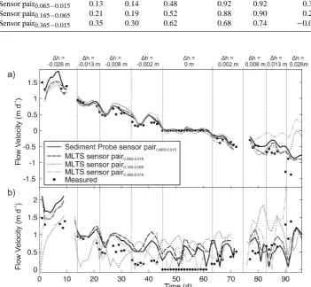
Darcian flow velocities of the sand box experiment were cal-culated using the analytical solutions of the 1-D heat trans-port Eqs. (1) and (2). As input the amplitude ratios and time lags derived from the three setups (Sediment Probe, MLTS and combined PBS and PCS) and calibrated thermal param-eter were used. Results of the shallow sensor pair0.065−0.015
(Fig. 6) will be discussed in detail within this section. The results of the other sensor pairs are presented in Table 4 for brevity. Flow velocities based on Sediment Probe am-plitude ratios (vSediment) ranged from 1.75 to −0.75 m d−1
and revealed a high accordance with the measured fluxes (RMSE = 0.13 m d−1,R2= 0.92) (Fig. 6a). The median of the normally distributed residuals between measured flow veloc-ities andvSedimentwas only−0.025 m d−1proving the
appro-priateness of the analytical solution based on Sediment Probe amplitude ratios.
Flow velocities based on MLTS derived amplitude ratios (vMLTS) also highly agreed with the experimentally measured
flow velocities (RMSE = 0.14 m d−1, R2= 0.92) (Fig. 6a). The median of the residuals between measured flow veloc-ities andvMLTSwas−0.046 m d−1.
The results show that vSediment and vMLTS were nearly
Table 4. Comparison of measured and calculated Darcian flow velocities based on Sediment Probe, MLTS and Piezometer Probe amplitude ratios and different temperature sensor spacings.
RMSE (m d−1) R2
Sediment MLTS Piezometer Sediment MLTS Piezometer
Probe Probe Probe Probe
Sensor pair0.065−0.015 0.13 0.14 0.48 0.92 0.92 0.39
Sensor pair0.165−0.065 0.21 0.19 0.52 0.88 0.90 0.28
Sensor pair0.365−0.015 0.35 0.30 0.62 0.68 0.74 −0.05
Fig. 6. Calculated Darcian flow velocities of sand box experiment using Keery’s amplitude ratio (a) and time lag method (b). Amplitude ratios and time lags were derived by temperature time series evaluation of Sediment Probe - sensor pair 0.065–0.015 and MLTS – sensor pairs 0.065–0.015, 0.165–0.065, 0.365–0.015.
arising from small differences in amplitude ratios be-tween both setups (Sect. 3.3.1). In contrast, the vertical flow velocities based on PBS and PBC amplitude ratios (vPiezometer) highly differed from the measured flow
veloc-ities (RMSE = 0.48 m d−1, R2= 0.39). The median of the residuals between measured flow velocities and vPiezometer
was −0.33 m d−1 and the distribution of residuals were slightly skewed. Thus, the calculated flow velocities based on PBS and PCS amplitude ratios were generally higher than the measured ones. These deviations were due to thermal ex-change processes within the piezometer pipes, which were not captured by the analytical solution. Despite the gen-eral overestimation ofvPiezometer, PBS and PCS amplitude
ratios could be used to distinguish between upward, no and
downward flow conditions, but they could not be reliably ap-plied to determine flow velocity magnitudes.
The results of sensor pair0.165−0.065and pair0.365−0.165
[image:12.595.119.471.148.472.2]-2 -1 0 1 2
Flow velocity (m d
)
-1
-2 -1 0 1 2
Flow velocity (m d
)
-1
0 20 40 60 80
Time (d)
0 20 40 60 80
Time (d)
c = 935 J kg K-1 -1
c = 1870 J kg K-1 -1
c = 2808 J kg K-1 -1
c = 935 J kg K ;-1 -1 = 2.35 W m K-1 -1
λe
c = 1870 J kg K ;-1 -1 = 4.75 W m K-1 -1
λe
c = 2808 J kg K-1 -1
;λe= 7.05 W m K
-1 -1
Δz= 0.025 m
Δz= 0.050 m
Δz= 0.075 m
λe= 2.35 W m K
-1 -1
λe W m K
-1 -1
= 4.75
λe W m K
-1 -1
= 7.05
no flow upward flow downward flow
downward flow no flow upward flow
d) c)
[image:13.595.127.468.65.292.2]b) a)
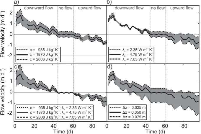
Fig. 7. Sensitivity of analytically calculated Darcian flow velocities to variations of heat capacity (a) and thermal conductivity (b), to simultaneous variations of heat capacity and thermal conductivity guaranteeing same thermal diffusivities (c) and to variations of temperature sensor spacing (d).
water fluxes would decrease the accuracy and limit the appli-cability of flux calculation using described temperature probe setups and analytical solutions.
Vertical flow velocities derived from the time lag method highly differed from the measured flow veloci-ties (Fig. 6b). The best fit was obtained for the Sed-iment Probe (RMSE = 0.78 m d−1, R2= -0.67) and MLTS
(RMSE = 0.87 m d−1, R2=−1.07). Again, PBS and PCS
showed the poorest fits (RMSE = 2.62 m d−1,R2=−16.57).
For all setups the time lag method was highly insensitive to small flow velocities and could not reflect measured flow ve-locities. Generally, the deviations between measured and cal-culated flow velocities of the Sediment Probe and MLTS de-creased with increasing flux magnitude (Fig. 6b). Therefore, flow velocities accurately calculated by time lag method need to be higher than at least 1.5 m d−1.
3.6 Sensitivity of calculated water flow velocities to sediment thermal properties and thermal dispersivity
The sensitivity analysis was based on the amplitude ratio method using the Sediment Probe - sensor pair0.065−0.015.
The calculated flow velocities (vSediment) were sensitive to
variations of heat capacity and thermal conductivity, to si-multaneous variations of heat capacity and thermal conduc-tivity preserving the same thermal diffusivities, and to varia-tions of temperature sensor distance.
The de- and increase of heat capacity resulted in an ab-solute de- and increase of vSediment, respectively. Thereby vSedimentwas more sensitive to variations of the heat
capac-ity during downward than during upward flow conditions (Fig. 7a). Under downward flow conditions, deep sediment temperatures were influenced by daily temperature varia-tions. In contrast, deep sediment temperatures were homo-geneous over time during upward fluxes. Thus, less heat was absorbed and released by quartz grains than during down-ward fluxes, decreasing the solutions sensitivity to saturated heat capacity.
The calculated flow velocity was nearly insensitive to vari-ations of thermal conductivity during downward flow con-ditions. For no-flow and upward flow conditions, a de-crease of thermal conductivity caused higher and an inde-crease of thermal conductivity caused lower estimates ofvSediment
(Fig. 7b). For upward flow conditions the direction of con-duction is directly opposed to heat advection. The system was dominated by advection, however, the propagation of the thermal signal was determined by conduction through the sediment particles, increasing the solution’s sensitivity to thermal conductivity.
As discussed for the optimisation of the thermal param-eters, during no-flow conditions, calculated vSediment was
(Fig. 7c). These deviations were caused by the superposition of the described variations ofvSedimentfor separated changes
of heat capacity and thermal conductivity (Fig. 7a and b). Absolute deviations of calculated flow velocities were highest for variations in temperature sensor spacing (Fig. 7d). Sensitivity analyses of calculated vSediment revealed the
need for an accurate estimation of thermal sediment prop-erties and temperature sensor spacing in order to accurately calculate vertical flow velocities. The omission of thermal dispersivity in the Keery et al.’s analytical solution of the 1-D heat transport equation (2007), might be a limitation when calculating vertical flow velocities. To test sensitivity of thermal diffusivity to vertical flow velocity, the Hatch et al.’s (2006) solution was used (vHatch). The calculated flow
velocities based on the Hatch amplitude ratio method were identical to the flow velocities calculated by Eq. (1), when the thermal dispersivity was set to zero. Also, vHatch
re-sults under consideration of thermal diffusivities in the range of solute dispersivity derived by conservative salt tracer ex-periment (Table 2) were similar to vKeery (maximum
devi-ation = 0.014 m d−1, RMSE = 0.0015 m d−1,R2= 0.99) with flow velocities ranging from−0.75 to 1.75 m d−1. Therefore, the baseline thermal diffusivity (about 10−6m2s−1) was one order of magnitude higher than the maximal thermal disper-sion coefficient (about 10−7m2s−1).
Our experimental results prove that the effect of thermal dispersion can be neglected for fine grained sediment and common water exchange fluxes between surface water and groundwater, when thermal dispersivity is equal to solute dispersivity.
4 Conclusions
Atmospheric temperature variations force the continuous transfer of energy between surface water and saturated sed-iment, thus forming subsurface temperature patterns deter-mined by water flux direction and magnitude. The applica-tion of the analytical soluapplica-tion of the 1-D heat transport equa-tion to observed temperature profiles provides a useful tool to quantify the water flux of saturated sediments. The accuracy of analytically calculated water fluxes was found to depen-dent on the temperature probe setup. Four temperature probe setups were installed into a sand box experiment to measure temporarily highly resolved vertical temperatures at depths of 0.015 m, 0.065 m, 0.165 m and 0.365 m under controlled exchange fluxes in the range of±1.3 m d−1.
Band pass filtering of the temperature records allowed ex-traction of the daily frequency, facilitating the use of analyt-ical solutions to calculate vertanalyt-ical water flux. Amplitude ra-tios of the direct temperature probe installation setups “Sedi-ment Probe” and “MLTS” significantly varied with sand box hydraulic gradients. These amplitude ratios provided an ac-curate basis for the analytical (amplitude ratio method) cal-culation of flow velocities in the range of−1.29 m d−1 to
+0.75 m d−1. Best results were obtained for small
temper-ature sensor distances close to the surface-subsurface inter-face (sensor pair0.065−0.015), guaranteeing that the shallow
thermal regime is driven by atmospheric temperature oscilla-tions and is independent of variable heat influx at the bottom of the sand box. Thermal properties of the medium-grained quartz sand were found to be 1870 J kg−1K−1for the heat capacity and 4.75 W m−1K−1for the thermal conductivity.
Calculated flow velocities were sensitive to thermal prop-erties of the saturated sediment and to sensor distance, but insensitive to thermal dispersivity equal to solute dispersiv-ity. Measured temperature profiles of indirect temperature probe installations as PBS and PCS were disturbed by ther-mal exchange processes within the piezometer pipes. The thermal exchange, independently occurring from the satu-rated sediment, restricted the sensitivity of amplitude ratios to the sandbox hydraulic gradients and to the calculated wa-ter flow velocities.
Time lags of all temperature probe setups were gener-ally insensitive to sand box hydraulic gradients, causing high deviations between measured and analytically (time lag method) calculated flow velocities in the range from −1.29 m d−1to 1.30 m d−1.
The interpretation of measured subsurface temperature data should contain a critical discussion of setup related ef-fects, as thermal exchange processes within piezometer pipes are independent of saturated sediment. The representation of saturated sediment temperatures is of main importance for the accurate quantification of subsurface water fluxes.
The experimental results support that, besides the Sedi-ment Probe, the MLTS setup can be used to accurately cal-culate vertical flow velocities. The advantage of MLTS is its installation into the saturated sediment, guaranteeing de-fined sensor distances. The lost cone installation of Sedi-ment Probe bears the potential to introduce deviations of de-fined temperature probe distances. The data of the MLTS setup can be accessed during operation by manually reading the sensor or via the GSM modem. The temperature data of TidbiTs directly installed into the sediment can only be ac-cessed after deinstallation. Data availability during operation enables the user to control the functioning of the setup and to promptly evaluate measurements. This prove the MLTS to be a valuable and appropriate tool for experimental ap-plication in natural streams to accurately quantify water and heat fluxes at the surface water-groundwater interface. The application along and across stream channels would provide highly resolved spatial and temporal information for better understanding the complex saturated sediment hydroecology.
Acknowledgements. We would like to thank Christian Anibas and an anonymous reviewer for their constructive remarks which helped to improve the quality of the paper.
References
Anderson, M. P.: Heat as a ground water tracer, Ground Water, 43, 951–968, 2005.
Anibas, C., Buis, K., Verhoeven, R., Meire, P., Batelaan, O.: A simple thermal mapping method for seasonal spatial patterns of groundwater-surface water interaction, J. Hydrol., 397, 93–104, doi:10.1016/j.jhydrol.2010.11.036, 2011
Bear, J.: Dynamics of Fluids in Porous Media, Elsevier, New York, 1972.
Boulton, A. J., Findlay, S., Marmonier, P., Stanley, E. H., and Valett, H. M.: The functional significance of the hyporheic zone in streams and rivers, Annu. Rev. Ecol. Syst., 29, 59–81, 1998. Bredehoeft, J. and Papadopolus, I. S.: Rates Of Vertical
Groundwa-ter Movement Estimated From the Earth’s Thermal Profile, Wa-ter Resour. Res., 1, 325–328, doi:10.1029/WR001i002p00325, 1965.
Cardenas, M. B.: Thermal skin effect of pipes in streambeds and its implications on groundwater flux estimation using di-urnal temperature signals, Water Resour. Res., 46, W03536, doi:10.1029/2009WR008528, 2010.
Carlslaw, H. S. and Jaeger, J. C.: Conduction of heat in solids, Clarendorn, Oxford, 2nd Edn., 1959.
Cirpka, O. A. and Kitanidis, P. K.: Characterization of mix-ing and dilution in heterogeneous aquifers by means of lo-cal temporal moments, Water Resour. Res., 36, 1221–1236, doi:10.1029/1999WR900354, 2000.
Cirpka, O. A. and Kitanidis, P. K.: Theoretical basis for the mea-surement of local transverse dispersion in isotropic porous me-dia, Water Resour. Res., 37, 243–252, 2001.
Conant, B.: Delineating and quantifying ground water discharge zones using streambed temperatures, Ground Water, 42, 243– 257, 2004.
Constantz, J.: Heat as a tracer to determine streambed
water exchanges, Water Resour. Res., 44, W00D10,
doi:10.1029/2008WR006996, 2008.
Constantz, J. and Stonestrom, D. A.: Heat as a tracer of water move-ment near streams, US Geological Survey, Circular 1260, 1–6, 2003.
Constantz, J., Thomas, C. L., and Zellweger, G.: Influence of di-urnal variations in stream temperature on stream flow loss and groundwater recharge, Water Resour. Res., 30, 3253–3264, 1994. Constantz, J., Tyler, S. W., and Kwicklis, E.: Temperature-Profile Methods for Estimating Percolation Rates in Arid Environments, Vadose Zone J., 2, 12–24, 2003.
de Marsily, G.: Quantitative Hydrogeology: Groundwater Hydrol-ogy for Engineers, 1st Edn., Elsevier, New York, 1986.
de Vries, D.: Thermal properties of soils, Physics of plant envi-ronment, 2nd Edn., North-Holland Publishing Co., Amsterdam, 1966.
Domenico, P. A. and Schwartz, F. W.: Physical and Chemical Hy-drogeology, 2nd Edn., John Wiley and Sons Inc., New York, 1990.
Hatch, C. E., Fisher, A. T., Revenaugh, J. S., Constantz, J., and Ruehl, C.: Quantifying surface water-groundwater in-teractions using time series analysis of streambed thermal records: Method development, Water Resour. Res., 42, W10410, doi:10.1029/2005WR004787, 2006.
Hopmans, J. W., Simunek, J., and Bristow, K. L.: Indirect estima-tion of soil thermal properties and water flux using heat pulse probe measurements: Geometry and dispersion effects, Water Resour. Res., 38, 1006, doi:10.1029/2000WR000071, 2002. Ingebritsen, S. E. and Sanford, W. E.: Groundwater in Geologic
Processes, Cambridge Univ. Press, New York, 1998.
Jensen, J. K. and Engesgaard, P.: Nonuniform Groundwater Dis-charge across a Streambed: Heat as a Tracer, Vadose Zone J., 10, 98–109, 2011.
Kalbus, E., Reinstorf, F., and Schirmer, M.: Measuring methods for groundwater - surface water interactions: a review, Hydrol. Earth Syst. Sci., 10, 873–887, doi:10.5194/hess-10-873-2006, 2006. Keery, J., Binley, A., Crook, N., and Smith, J. W. N.: Temporal and
spatial variability of groundwater-surface water fluxes: Develop-ment and application of an analytical method using temperature time series, J. Hydrol., 336, 1–16, 2007.
Krause, S., Hannah, D. M., Fleckenstein, J. H., Heppell, C. M., Kaeser, D., Pickup, R., Pinay, G., Robertson, A. L., and Wood, P. J.: Inter disciplinary perspectives on processes in the hyporheic zone, Ecohydrology, 4, 481-499, 2011.
Lapwood, E. R.: Convection Of A Fluid In A Porous Medium, Proc. Cambridge Philos. Soc., 44, 508–521, 1948.
Lautz, L. K.: Impacts of nonideal field conditions on vertical wa-ter velocity estimates from streambed temperature time series, Water Resour. Res., 46, W01509, doi:10.1029/2009WR007917, 2010.
Rau, G. C., Andersen, M. S., McCallum, A. M., and Acworth, R. I.: Analytical methods that use natural heat as a tracer to quantify surface water-groundwater exchange, evaluated us-ing field temperature records, Hydrogeol. J., 18, 1093–1110, doi:10.1007/s10040-010-0586-0, 2010.
Rosenberry, D. O. and LaBaugh, J. W.: Field Techniques for Esti-mating Water Fluxes Between Surface Water and Ground Water, US Geological Survey, Techniques and Methods 4-D2, 2008. Schmidt, C., Bayer-Raich, M., and Schirmer, M.:
Characteriza-tion of spatial heterogeneity of groundwater-stream water in-teractions using multiple depth streambed temperature measure-ments at the reach scale, Hydrol. Earth Syst. Sci., 10, 849–859, doi:10.5194/hess-10-849-2006, 2006.
Schmidt, C., Conant, B., Bayer-Raich, M., and Schirmer, M.: Evaluation and field-scale application of an ana-lytical method to quantify groundwater discharge using mapped streambed temperatures, J. Hydrol., 347, 292–307, doi:10.1016/j.jhydrol.2007.08.022, 2007.
Sch¨on, J.: Physical Properties of Rocks: Fundamentals and Princi-ples of Petrophysiks, 2nd Edn., Porgamon, Oxford, 1998. Schornberg, C., Schmidt, C., Kalbus, E., and Fleckenstein, J. H.:
Simulating the effects of geologic heterogeneity and transient boundary conditions on streambed temperatures – Implications for temperature-based water flux calculations, Adv. Water Re-sour., 33, 1309, doi:10.1016/j.advwatres.2010.04.007, 2010. Silliman, S. E., Ramirez, J., and McCabe, R. L.: Quantifying
Down-flow Through Creek Sediments Using Temperature Time-Series – One-Dimensional Solution Incorporating Measured Surface-Temperature, J. Hydrol., 167, 99–119, doi:10.1016/0022-1694(94)02613-G, 1995.
Sophocleous, M.: Interactions between groundwater and surface water: the state of the science, Hydrogeol. J., 10, 52–67, 2002. Stallman, R. W.: Steady 1-Dimensional Fluid Flow In A
Semi-Infinite Porous Medium With Sinusoidal Surface Temperature, J. Geophys. Res., 70, 2821, doi:10.1029/JZ070i012p02821, 1965. Stonestrom, D. A. and Blasch, K. W.: Determining temperature
and thermal properties for heat-based studies of surface-water ground-water interactions, US Geological Survey, Circular 1260, 73–80, 2003.
Storey, R. G., Howard, K. W. F., and Williams, D. D.: Fac-tors controlling riffle-scale hyporheic exchange flows and their seasonal changes in a gaining stream: A three-dimensional groundwater flow model, Water Resour. Res., 39, 1034, doi:10.1029/2002WR001367, 2003.
Suzuki, S.: Percolation Measurements Based On Heat Flow Through Soil With Special Reference To Paddy Fields, J. Geo-phys. Res., 65, 2883–2885, 1960.
Turcotte, D. L. and Schubert, G.: Geodynamics: Application of Continuum Physics to Geologic Problems, John Wiley and Sons, New York, 1982.
Tyler, S. W., Selker, J. S., Hausner, M. B., Hatch, C. E., Torgersen, T., Thodal, C. E., and Schladow, S. G.: Environmental tem-perature sensing using Raman spectra DTS fiber-optic methods, Water Resour. Res., 45, W00D23, doi:10.1029/2008WR007052, 2009.
van Wijk, W. and de Vries, D.: Periodic temperature variations in a homogeneous soil, in: Physics of plant environment, 2nd Edn., North-Holland Publishing Co., Amsterdam, 1966.
Vogt, T., Schneider, P., Hahn-Woernle, L., Cirpka, O. A.: Estima-tion of seepage rates in a losing stream by means of fiber-optic high-resolution vertical temperature profiling, J. Hydrol., 380, 154–164, doi:10.1016/j.jhydrol.2009.10.033, 2010.