www.hydrol-earth-syst-sci.net/15/2805/2011/ doi:10.5194/hess-15-2805-2011
© Author(s) 2011. CC Attribution 3.0 License.
Earth System
Sciences
Towards reconstruction of the flow duration curve:
development of a conceptual framework with a physical basis
Y. Yokoo1and M. Sivapalan2,3
1Faculty of Symbiotic Systems Science, Fukushima University, Fukushima, Japan
2Department of Civil and Environmental Engineering, University of Illinois at Urbana-Champaign, Illinois, USA 3Department of Geography, University of Illinois at Urbana-Champaign, Illinois, USA
Received: 28 March 2011 – Published in Hydrol. Earth Syst. Sci. Discuss.: 20 April 2011 Revised: 24 August 2011 – Accepted: 1 September 2011 – Published: 9 September 2011
Abstract. In this paper we investigate the climatic and land-scape controls on the flow duration curve (FDC) with the use of a physically-based rainfall-runoff model. The FDC is a stochastic representation of the variability of runoff, which arises from the transformation, by the catchment, of within-year variability of precipitation that can itself be char-acterized by a corresponding duration curve for precipita-tion (PDC). Numerical simulaprecipita-tions are carried out with the rainfall-runoff model under a variety of combinations of cli-matic inputs (i.e. precipitation, potential evaporation, includ-ing their within-year variability) and landscape properties (i.e. soil type and depth). The simulations indicated that the FDC can be disaggregated into two components, with sharply differing characteristics and origins: the FDC for sur-face (fast) runoff (SFDC) and the FDC for subsursur-face (slow) runoff (SSFDC), which included base flow in our analysis. SFDC closely tracked PDC and can be approximated with the use of a simple, nonlinear (threshold) filter model. On the other hand, SSFDC tracked the FDC that is constructed from the regime curve (i.e. mean monthly runoff), which can be closely approximated by a linear filter model. Sensitivity analyses were carried out to understand the climate and land-scape controls on each component, gaining useful physical insights into their respective shapes. In particular the results suggested that evaporation from dynamic saturated areas, es-pecially in the dry season, can contribute to a sharp dip at the lower tail of the FDCs. Based on these results, we develop a conceptual framework for the reconstruction of FDCs in un-gauged basins. This framework partitions the FDC into: (1) a fast flow component, governed by a filtered version of PDC, (2) a slow flow component governed by the regime curve, and (3) a correction to SSFDC to capture the effects of high evapotranspiration (ET) at low flows.
Correspondence to: Y. Yokoo
1 Introduction
The flow duration curve (FDC) is a representation of the frequency distribution of streamflow of a specific time pe-riod (normally daily, but can also be hourly) (see Vogel and Fennessey, 1994, 1995; Smakhtin, 2001). It is effectively an alternative representation of the cumulative distribution function of daily (or hourly) streamflow. Hydrologists have traditionally analyzed the FDC using purely graphical rep-resentations (Ward and Robinson, 1990), or using stochastic models that focus on fitting appropriate statistical distribu-tions and estimating associated parameters (see most recent work by Castellarin et al., 2004a; Iacobellis, 2008). Many of the past efforts have focused on relating the characteristics of the FDCs (e.g. shape measures or parameters of the statistical distributions, as the case may be), to the catchment’s climatic and physiographic characteristics, to assist in regionalization of the FDCs and as a precursor to estimation in ungauged catchments.
2806 Y. Yokoo and M. Sivapalan: Towards reconstruction of the flow duration curve globally applicable relationships. In other words, if one were
to think of the several empirical studies reviewed above as pieces of a jigsaw puzzle, we have not yet acquired the under-standing and the methodology to complete that puzzle. The work presented in this paper is a small step in developing a general process-based characterization of the FDC, fully reflecting the complex interactions between climate (i.e. pre-cipitation and radiation) and catchment physiographic char-acteristics that contribute to the generation of runoff by many different mechanisms.
In recent times there have been several promising efforts that approach FDCs from a process perspective. Castel-larin et al. (2004a) proposed a new stochastic representa-tion of FDCs to reproduce the observed variance of an-nual flows. Botter et al. (2007a) presented the mathemat-ical formalisms for the derivation of the probability dis-tribution (which is equivalent to FDCs), associated with within-year variation of the baseflow component of daily streamflow. Botter et al. (2007b) derived the FDCs using a stochastic-dynamic model that captured the interaction of within-year sequences of precipitation events with a simple lumped model of subsurface drainage, which is governed by a field capacity threshold and a characteristic catchment res-idence time. The model was successfully tested in a number of catchments across the United States. Yilmaz et al. (2008) approached the same question with the use of the Sacramento Soil Moisture Accounting Model (SAC-SMA) and explored, through sensitivity analyses, the effect of the upper layer ten-sion water capacity (which is a model parameter) and other model parameters on the shape of FDCs, including the rela-tive extents of the high flow segment and the low flow seg-ment, and the slope of intermediate flow segment. Botter et al. (2009) later extended their probabilistic model to explain observed catchment streamflow regimes across the United States. Muneepeerakul et al. (2010) further extended the stochastic-dynamic model of Botter et al. (2007a,b, 2009) to include fast runoff processes, and in this way presented a stochastic framework to mimic the within-year variability of both fast and slow flow components of the FDCs in a number of US catchments.
The work presented in this paper can be viewed as a fur-ther extension of the work of Botter et al. (2007a,b, 2009) and Muneepeerakul et al. (2010) but is different from their work in several ways: (i) this numerical modeling study will use a more advanced physically-based, continuous water bal-ance model that includes runoff generation by several mech-anisms; (ii) being a numerical model, the simulations will be able to capture the effects of not only the randomness of pre-cipitation events (i.e. the Poisson assumption made in Botter et al., 2007a,b) but also, explicitly, the effects of systematic seasonal variability of both precipitation and potential evap-oration, which together govern the variability of antecedent soil moisture conditions and their effects on runoff gener-ation; and (iii) the model used is a lumped quasi-2D model, and does include lateral flow processes (e.g. saturation excess
overland flow and subsurface stormflow), and can therefore be used to assess their relative effects on the shape of the FDCs.
The water balance model used here is taken from Yokoo et al. (2008). This model was developed on the basis of governing equations for mass and momentum balance de-rived at the scale of a representative elementary watershed (REW), which have been the basis of numerous distributed modeling efforts (e.g. Zhang and Savenije, 2005; Zehe et al., 2006; Lee et al., 2007; Li et al., 2011; Li and Sivapalan, 2011). Previous applications of the model used here have involved the exploration of (1) mean annual water balance within the Budyko (1974) framework (Reggiani et al., 2000), and (2) mean monthly runoff (i.e. regime curve) (Yokoo et al., 2008), with both studies including the partitioning into surface and subsurface runoff as well. The current paper thus represents a further application of the model to develop in-sights into the FDC. The main aims of the paper are: (1) To generate insights into the shape of the FDCs, and to deter-mine the relative controls of climate and landscape properties on the FDCs, including its various components; (2) to de-velop a conceptual framework that can be utilized, in combi-nation with the insights gained into the climate and landscape controls on the FDCs, to help reconstruct FDCs in ungauged basins.
2 Methodology
The key components of the methodology involve the use of (i) a stochastic rainfall model to generate synthetic rain-fall event sequences, under different assumed climates, and (ii) the lumped quasi-2-D, physically based rainfall-runoff model. The two models are used in sequence for a variety of combinations of soils and climate to generate runoff time series (including surface and subsurface runoff components) from which the FDCs are derived, including its two compo-nents. Next we present the brief summaries of the rainfall and rainfall-runoff models.
2.1 Stochastic rainfall model
We employ an event-based stochastic model of precipitation time series developed by Robinson and Sivapalan (1997) to generate multiple random realizations of synthetic precipita-tion inputs. This model is capable of reproducing multi-scale temporal variability of rainfall intensities, including random within-storm and between-storm variability, the parameters of which can, if needed, vary seasonally in a deterministic manner. Both storm durations and inter-storm periods are as-sumed to follow the exponential distribution, the parameters of which also vary sinusoidally over the year. Mean rain-fall intensities during storms are assumed to follow a condi-tional gamma distribution, subject to the chosen storm du-ration, the parameters of which could also vary sinusoidally over the year. The mean storm intensity is further disaggre-gated to hourly intensity patterns (within-storm patterns) us-ing stochastically generated mass curves (Huff, 1967; Chow et al., 1988). This disaggregation is carried out with the use of the random cascade model (Koutsoyiannis and Foufoula-Georgiou, 1993): the random weights chosen to sequentially disaggregate the rainfall depth at finer time steps are assumed to follow the beta distribution.
Details of the synthetic rainfall model can be found in the original paper by Robinson and Sivapalan (1997). For convenience, the model parameters used for the simulations reported in this paper are the same as those in Table 2 of Robinson and Sivapalan (1997), derived for the raingauge at Salmon Creek in Western Australia (which is used mainly for convenience). In this study we generated hourly rainfall intensities for a period of 13 years, which were then rescaled so that the mean annual rainfall over the 13 year period be-comes approximately 1000 mm, consistent with the notion that this is a completely theoretical study. In the simulation results presented in this paper, we used 3 year-long segment of the synthetic rainfall timeseries, which includes the effect of inter-annual variability of annual rainfall, as well within-year variability at the event scale.
The attraction of using such a model for generating syn-thetic precipitation inputs is that it allows us to perform diag-nostic analyses whereby we can switch on and off different components of the natural variability, and investigate their
1
y
s
z
r
z
s
P
Q
s
ET
PET
Q
ss
P
I
u
I
s
C
L
h
Datum
Z
OF
1
2
Figure 1. 3
4
Fig. 1. Conceptual drawing of Reggiani et al.’s (2000) REW-scale water balance model: P: Precipitation, ET: Evapotranspiration, PET: Potential evapotranspiration,Qs: Surface runoff,Qss: Sub-surface runoff,Iu: Infiltration from the ground surface,Is:
Infil-tration to the saturated zone,C: Capillary rise, OF: Outflow from saturated zone,Z: Average elevation of ground surface from datum, zr: Average elevation of channel bed with respect to datum,zs: Av-erage elevation of the bottom surface of the REW with respect to datum,ys: Average thickness of saturated zone,Lh: Averaged hor-izontal length of one side of REW.
effects on the shape of the FDCs. This is a significant advan-tage over the use of historical data.
2.2 Water balance model
[image:3.595.322.535.62.243.2]2808 Y. Yokoo and M. Sivapalan: Towards reconstruction of the flow duration curve et al. (2008). In this paper we only give a brief outline of the
model and the parameter sets used in the simulations reported here.
2.2.1 Governing equations
The water balance model by Reggiani et al. (2000) consists of three coupled governing equations: mass balance in the un-saturated zone, momentum balance in the unun-saturated zone, and mass balance in the saturated zone, as shown in Eqs. (1)– (3), respectively.
ρε d
dt (suyuωu)
| {z }
Change in unsaturated storage
(1)
= min
ρP ωu,
ρKsωu
3u 1
2 yu −ψu
·δ [0, tr]
| {z }
Infiltration
+ ρεωuvu
| {z }
Percolation or capillaryrise
−ρωu 1
R (tanh 5su)
1.0 +R−5−(1/5)PET·δ[tr, tm]
| {z }
Evapotranspiration
− ερg suyuωu
| {z }
Gravitational force
(2)
+ ερg suωu 1
2 yu −ψu
| {z }
Force acting onthe water across the land surface
= K−1ερg yuωuvu
| {z }
Resistance force
ρε d
dt (ysωs)
| {z }
Change in the saturated storage
= − ρεωuvu
| {z }
Percolation or capillary rise
(3)
− ρKsωo
cos(γo) 3s
1
2 (ys −zr +zs)
| {z }
Outflow across seepage faces
.
The functionδ[0, tr] (δ[tr, tm])in Eq. (1) is equal to 1 (0)
if time t in a meteorological period, which consists of a storm duration and the subsequent inter-storm period, falls between 0 (tr) andtr(tm) during a storm period, and is zero
(Eq. 1) otherwise during the inter-storm period. The vari-ablessu, yu, ωu, 3u, ψu, vu, K, P, and PET are,
respec-tively, saturation degree in the unsaturated zone, average thickness of the unsaturated zone, unsaturated surface area fraction, a characteristic length scale for infiltration, pres-sure head in the unsaturated zone, upward velocity in the
unsaturated zone, unsaturated hydraulic conductivity, precip-itation intensity, and a seasonally-varying potential evapora-tion. The variablesys,ωs,ωo,γo, and3s are, respectively,
[image:4.595.46.282.163.594.2]the average thickness of the saturated zone, area fraction of the saturated zone kept at 1.0 based on the assumption that a saturated zone exists everywhere below the water table of a REW, the saturated surface area fraction is assumed to vary with the saturation degree of the unsaturated zone, slope an-gle of the overland flow plane with respect to horizontal, and a typical length scale for seepage outflow. The definitions of the other variables used in these equations are summarized in Table 1 as well as in the appendix of Reggiani et al. (2000). These equations contain 7 unknowns, and therefore 4 addi-tional closure relations are required. Most of those are simple geometric relations, but the parameterization of the seepage area fractionωois a non-trivial one requiring further
assump-tions, as outlined below: ωo =
ys −zr +zs
Z −zr +zs
(4)
˙
ωo = − ˙ωu. (5)
In Eq. (4),Zis the average thickness of the subsurface zone, zris channel bed elevation with respect to a datum,zsis the
average elevation of the bottom surface of the REW with re-spect to the datum,ysis the average thickness of the
subsur-face zone along the vertical, andωuis the area fraction of the
unsaturated zone.
To solve the governing equations, we need constitutive re-lationships regarding the hydraulic properties of the soil. We use the VK model for hydraulic conductivity (Kosugi, 1994) for the water retention curve, which has the advantage that it does not have a discontinuous point near saturation, con-tains only three physical parameters, and thus permits easy calibration to measured water retention data. Equations (6) or (7) are the functional forms of the VK model,
ψu = (
ψc − (ψc−ψ0)· n(s
u)−1/m−1.0 m
o1.0−m
(su <1.0)
ψc (su =1.0)
(6)
su =
1/
1 +mψc−ψu
ψc−ψ0
1/(1−m)m
(ψu < ψc)
1.0 (ψu ≥ ψc)
(7)
whereψc,ψ0, and mare bubbling pressure, capillary
pres-sure at the inflection point on the su−ψu curve, and
di-mensionless parameter, respectively. For the unsaturated hy-draulic conductivity K, we use Eq. (8) from Reggiani et al. (2000), which was in turn taken from (Brutsaert, 1966),
K = Ks · (su)λ (8)
Table 1. Meaning, values and the ranges of model parameters used in the numerical experiments.
Group Name Description (unit) Value and the range
Climate Pa Annual precipitation (mm) 1000 (mean)
R Dryness index 0.5 (0.0–2.0)
PETa Potential evapotranspiration (mm) Pa·R
Geographic Z Depth of soil layer (m) 5–20
zr Average elevation of channel bed from datum (m) 3.0–7.0
zs Average elevation of the bottom end of REW from datum (m) 0
ys Average thickness of saturated zone (m) Z−yuωu, 0.5Z(ini.3)
yu Average thickness of unsaturated zone (m) (Z−ys)/ωu
ωu Unsaturated surface area fraction of unsaturated zone (Z−ys)/yu
ωo Saturated surface area fraction of unsaturated zone 1−ωu
ωs Horizontal area fraction of saturated zone 1
su Saturation degree of unsaturated zone 0.5 (ini.3)
3u Typical length scale for infiltration suyu
3s Typical length scale for seepage outflow (m) 10
γo Slope gradient of the overland flow plane, which is assumed to be nearly flat. 0.0
Lh Representative hillslope length of a REW in Fig. 1 (m) 500
G Slope gradient of a REW 0.002–0.010
Soil K Hydraulic conductivity (m s−1) –
Ks Saturated hydraulic conductivity (m s−1)1 Silty loam 3.4×10⁻⁶ Sandy loam 3.4×10⁻⁵ Sand 8.6×10⁻⁵
λ Pore-disconnectedness index1 Silty loam 4.7 Sandy loam 3.6 Sand 3.4
ε Porosity1 Silty loam 0.35
Sandy loam 0.25 Sand 0.20
m Dimensionless parameter related to the width of the pore radius distribution2 Silty loam 0.44 Sandy loam 0.70 Sand 0.77
ψc Bubbling pressure (m)2 Silty loam −0.20
Sandy loam −0.10 Sand −0.10
ψ0 Capillary pressure at the inflection point on theθ−ψcurve (m)2 Silty loam −0.30 Sandy loam −0.25 Sand −0.16
ψu pressure head in the unsaturated zone –
vu Velocity in the unsaturated zone (m s−1), positive when directed upward. –
Others ρ Water density (kg m−3) 1000
g Gravitational acceleration (m s−2) 9.80
t Time –
The1indicates parameters are taken from Bras (1990), and the2indicates the parameters are obtained by calibration. The calibration involved manually adjusting the parameters
in Kosugi’s (Kosugi, 1994) water retention curve (VK model) with those from the Brooks-Corey model (Brooks and Corey, 1966) and the parameters in Bras (1990) as much as
possible. The3indicates initial condition.
2.2.2 Numerical solution of governing equations and water balance calculations
In solving the governing equations, we need to provide initial conditions for the saturation degree in the unsaturated zonesu
and water table thicknessys, in addition to parameter settings
for soil properties, climatic inputs, and the two geometric
parameters ofγo and3s in Table 1. Arbitrary initial
val-ues for soil moisture and water table depth are appropriate so long they are not very different from physically acceptable values. We set the initial values of 0.5 forsuandzr−zs for
ys, in common to all the numerical experiments. The soil
2810 Y. Yokoo and M. Sivapalan: Towards reconstruction of the flow duration curve and3s, are taken to be 0.0 and 10 m, respectively. For the
cli-matic inputs, we assumed the annual rainfall to be 1000 mm and annual potential evaporation was then chosen on the ba-sis of the climatic dryness indexR, the ratio of annual poten-tial evaporation over annual precipitation, given by:
R = PETa
Pa
(9) where PETa and Pa are annual evaporation (m) and
an-nual precipitation (m), respectively. For reference, Table 1 presents the list of all the parameters and the ranges of val-ues used in this paper.
In this paper we utilize a fourth-order Runge-Kutta inte-gration method for solving the coupled governing equations simultaneously. Firstly, we gave initial condition forsuand
ysto solve Eq. (2) as mentioned above. Secondly, we solved
Eqs. (1) and (3) to obtainsu andys in the next step of the
Runge-Kutta integration method. The simulations were car-ried out for a period of 13 years with a time step of 5 min. Only the last 3 years of the runoff time series produced by the model were used to estimate the FDCs; in this way, the effect of initial conditions on the resulting FDCs can be ne-glected. Although we cannot completely remove the effect of initial conditions, we visually confirmed that the effect was negligible. We also confirmed that seasonal variability is strong enough in the 3 year long runoff time series whenever climatic seasonality is active in the climatic setting, through setting the seasonal amplitudes ofP and PET to be respec-tively equal to their mean values.
2.3 Setup for the numerical experiments
The main analysis we perform in this paper is a series of numerical experiments with the numerical model of water balance. These experiments take the form of sensitivity anal-yses with the rainfall-runoff model to investigate the controls of climate, soil, and topography on the shapes of the FDCs, including the SFDCs (surface runoff) and SSFDCs (subsur-face stormflow). Average annual precipitationPawas set to
1000 mm in all of the simulations. The synthetically gen-erated precipitation time seriesP (t )based on the stochastic model of Robinson and Sivapalan (1997) are used in all the simulations. Dryness index R was varied from 0.5 to 1.5 by changing the annual potential evapotranspiration PET(t), with bothP (t ) and PET(t) including seasonal variabilities that are perfectly in-phase or perfectly out-of-phase. We also consider three different soil types: silty loam, sandy loam, and sand; assumed soil depths ranged from 6 m to 8 m.
3 Results
3.1 FDC separation into constituent elements
Our goal in this paper is to use carefully defined rainfall-runoff simulations to elucidate the physical meaning of the
1 1.0E-02
1.0E-01 1.0E+00 1.0E+01 1.0E+02
0.00 0.25 0.50 0.75 1.00
Fl
u
x(
mm/
d
) /
Qm(
m
m/
d
)
Exceedance Probability nQ nQs nQss nMQ nP
1 2
Figure 2. 3
4
Fig. 2. An example of the decomposition of the flow duration curve normalized by mean annual daily flowQm. “nQ”, “nQs”, “nQss”, “nP” are normalized duration curves of daily flow, daily surface flow, daily subsurface flow, and daily precipitation; “nMQ” is flow duration curve associated with the regime curve - ensemble aver-aged mean within-year daily flow variation normalized by mean an-nual daily flowQm). We calculated exceedance probabilities for
nQ, nQs, nQss, and nP as the order numbers sorted by their
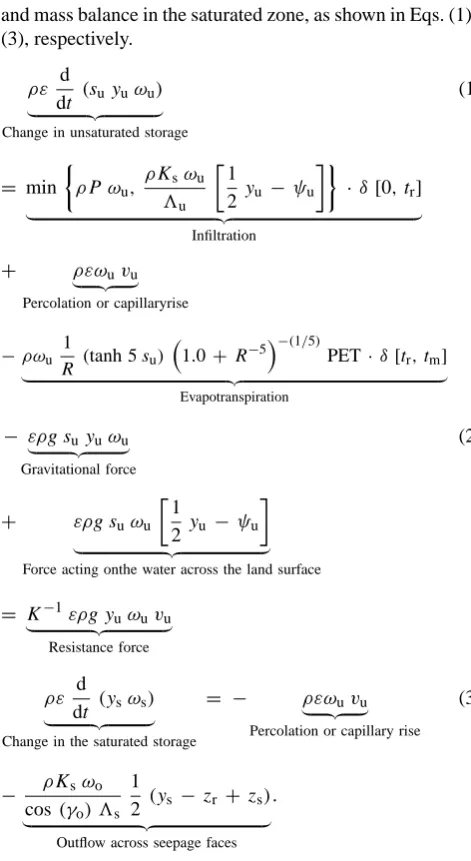
mag-nitudes for a total of 3 years divided by 1096 which is 365×3 + 1. For the exceedance probability of nMQ, we calculated the sorted or-der of the mean monthly flow divided by 13 which is 12 + 1. Hence, precipitation and surface flow occurred about 1/3 of the total calcu-lation period and subsurface flow appeared every time period. Dry-ness index is 0.5, and seasonal peaks of precipitation and potential evapotranspiration are in phase making a humid summer climate. Soil type is set as silty loam. Soil depth is 8 m. Surface gradient is 0.006.
shape of the FDC in terms of its underlying process con-trols. Figure 2 shows the result of a test run for a hypo-thetical watershed (with default parameters – slope gradient of 0.006, soil type: silty loam, soil depth is 8 m), in a hu-mid climate with the seasonality of P and PET that are in phase. In this case the FDC (thick black curve) is presented along with the surface flow duration curve (SFDC, thin blue curve) and the subsurface flow duration curve (SSFDC, thin red curve). We can clearly see that the upper tail of the FDC is quite close to that of the SFDC, whereas the middle sec-tion and the lower tail of the FDC track well the SSFDC. In addition, we can see that SFDC is a filtered version of the precipitation duration curve (PDC). Likewise we can see that the SSFDC closely tracks (is slightly below) the FDC of the mean monthly runoff (i.e. the regime curve). This is sugges-tive of the potential of constructing the middle part and lower tail of the FDC from the regime curve.
[image:6.595.319.534.65.198.2]literature as well (e.g. Vogel and Fennessey, 1995; Smakhtin, 2001; Castellarin et al., 2004a).
In the sections below we will present results of simulations for several combinations of climate and soils to confirm that the breakdown suggested above remains valid in all or most cases. If these features persist for all combinations of climate and landscape properties, this would then present an elegant and physically meaningful way to perform the separation of the FDC into its two component building blocks. In addi-tion, we will explore the climatic and landscape (i.e. soils) controls on the two building blocks.
3.2 Sensitivity of the FDC to climate factors
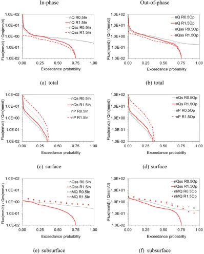
The initial set of simulations involves different combina-tions of climate variability, which are the principal drivers of runoff variability. As shown in Fig. 3 four different cases are considered. Two different values of climatic dryness (de-fined as PET/P) are assumed, namely 0.5 (humid) and 1.5 (arid), to be consistent with the literature (i.e. Farmer et al., 2003; Mohamoud, 2008). In each case, two different types of seasonality are assumed, i.e. in-phase and out-of-phase sea-sonality ofP and PET. Apart from these default values of soil type (silty loam), a soil depth of 8 m, and the topographic gradient of 0.006 are assumed. Figure 3a, c and e are for the case for in-phase seasonality, whereas Fig. 3b, d and f are for out-of-phase seasonality. Figure 3c and d present the FDCs for surface runoff, whereas Fig. 3e and f present the FDCs for subsurface runoff.
Figure 3a and b present the FDCs forR= 0.5 (humid) and 1.5 (arid), and the corresponding FDCs for the subsurface flow component (SSFDC) whereP and PET are in phase a and out-of-phase b. The results show that, in both cases, the middle section and the lower tail of the FDCs very well track the SSFDC. The FDCs deviate from the SSFDCs towards the upper tail, which is suggestive of surface runoff compo-nent. This leads to the FDCs of the surface runoff component (SFDC), which are presented in Fig. 3c and d, along with the FDCs of the precipitation inputs (PDC). The results reflect the presence of an infiltration loss, with a larger loss term in the arid case, and a smaller loss in the humid case, with sea-sonality not having a significant impact. The transformation between the PDC and SFDC are suggestive of a nonlinear (threshold) filter.
Figure 3e and f present the model generated FDC for sub-surface runoff (SSFDC) for bothR= 0.5 andR= 1.5. Along with these, we also present the corresponding FDCs associ-ated with the simulassoci-ated regime curve. The results indicate that the FDCs derived from the regime curve approximate the SSFDCs in a humid climate, regardless of climatic sea-sonality. However, in the arid climate where ET becomes the dominant process, the SSFDCs deviate from the FDCs derived from the regime curves, especially for low flows, re-sulting in a sharp dip in the FDCs towards the lower tail. Indeed, in arid climate with out-of-phase seasonality, there
is a slight dip in the FDC of the regime curve as well to-wards the lower tail. The difference between the FDCs and the monthly runoff FDC (equivalent to the regime curve) is due to the presence or absence of temporal averaging. We would need an additional transfer function to reproduce the shape of the lower part of a FDC from the FDCs of monthly runoff (i.e. regime curve).
3.3 Sensitivity of the FDCs to soil type
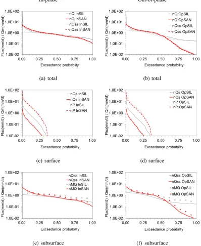
Figure 4 shows the results of sensitivity analyses with re-spect to soil type and climatic seasonality (in-phase and out-of-phase). Otherwise, these simulations use default values of climate dryness ofR= 0.5 (humid), a soil depth of 8m and a topographic gradient of 0.006. As shown in Fig. 4 four differ-ent cases are considered: sand vs. silty loam (sandy soils with intermediate hydraulic properties are omitted for simplicity), and in-phase vs. out-of-phase seasonality. Figure 4a, c and e are for the case for in-phase seasonality, whereas Fig. 4b, d and f are for out-of-phase seasonality. Figure 4c and d present the FDCs for surface runoff, whereas Fig. 4e and f present the FDCs for subsurface runoff.
Figure 4a and b present the FDCs for two different types of soil (sand and silty loam), and the corresponding FDCs for the subsurface flow component (SSFDC). The results show that, in both cases, the middle section and the lower tail of the FDCs almost perfectly track the SSFDC. The FDC for sand deviates from that for silty loam in the lower tail in the case of in-phase seasonality; the deviations are much more in the case of out-of-phase seasonality. In either case, the net result is that the FDC for sand is steeper than those for silty loam. These results suggest that a combination of out-of-phase sea-sonality and well drained soils push the response towards ephemeral systems. The FDCs deviate from the SSFDCs to-wards the upper tail for silty loam (suggesting that the devia-tion is due to surface runoff due to infiltradevia-tion excess runoff). Interestingly, in the case of sand, there is very little devia-tion between the FDC and SSFDC for the entire range of flows, suggesting that subsurface flow makes a contribution to high flows as well. This leads us to look at the FDCs of the surface runoff component (SFDC), which are presented in Fig. 4c and d, along with the FDCs of the precipitation inputs (PDC). The difference reflects infiltration loss, with larger loss in sand.
Figure 4e and f present the model generated FDCs for sub-surface runoff (SSFDC) along with the corresponding FDCs associated with the regime curve. The results indicate that the FDCs derived from the regime curve nicely track the SSFDCs in a humid climate, regardless of climatic season-ality. However, in the case of out-of-phase seasonality, the FDCs for sand deviate from those for silty loam.
2812 Y. Yokoo and M. Sivapalan: Towards reconstruction of the flow duration curve
1
1
In-phase Out-of-phase
1.0E-02 1.0E-01 1.0E+00 1.0E+01 1.0E+02
0.00 0.25 0.50 0.75 1.00
Fl
ux
(m
m
/d)
/
Q
m
(m
m
/d
)
Exceedance probability nQ R0.5In nQ R1.5In nQss R0.5In nQss R1.5In
(a)
total
1.0E-02 1.0E-01 1.0E+00 1.0E+01 1.0E+02
0.00 0.25 0.50 0.75 1.00
Fl
ux
(m
m
/d
) /
Q
m
(m
m
/d)
Exceedance probability nQ R0.5Op nQ R1.5Op nQss R0.5Op nQss R1.5Op
(b)
total
1.0E-02 1.0E-01 1.0E+00 1.0E+01 1.0E+02
0.00 0.25 0.50 0.75 1.00
Fl
ux
(m
m
/d
) /
Qm
(m
m/
d)
Exceedance probability nQs R0.5In nQs R1.5In nP R0.5In nP R1.5In
(c)
surface
1.0E-02 1.0E-01 1.0E+00 1.0E+01 1.0E+02
0.00 0.25 0.50 0.75 1.00
Fl
ux
(m
m
/d
) /
Qm
(m
m/
d)
Exceedance probability nQs R0.5Op nQs R1.5Op nP R0.5Op nP R1.5Op
(d)
surface
1.0E-02 1.0E-01 1.0E+00 1.0E+01 1.0E+02
0.00 0.25 0.50 0.75 1.00
Fl
ux
(m
m
/d)
/
Qm(
m
m
/d)
Exceedance probability nQss R0.5In nQss R1.5In nMQ R0.5In nMQ R1.5In
(e)
subsurface
1.0E-02 1.0E-01 1.0E+00 1.0E+01 1.0E+02
0.00 0.25 0.50 0.75 1.00
F
lux
(m
m
/d)
/
Q
m
(m
/d
)
Exceedance probability nQss R0.5Op nQss R1.5Op nMQ R0.5Op nMQ R1.5Op
(f)
subsurface
2
Figure 3.
3
4
Fig. 3. Effect of dryness indexR on the FDC for different types of climatic seasonality: (a), (b): Total flow FDC, (c), (d):surface flow FDC, (e), (f): subsurface flow FDC. (a), (c), (e): seasonal peaks ofP and PET are in phase, (b), (d), (f): seasonal peaks ofP and PET are of opposite phase. The numbers afterRare dryness indices. In each panels, “In” and “Op” indicatesP and PET are in-phase and of out-of-phase, respectively. Qmis mean annual daily flow (mm d−1). “nMQ” refers to FDC associated with the regime curve – ensemble averaged mean within-year daily variation normalized by mean annual daily flowQm. Default value of soil type is silty loam, soil depth is 8 m, and the topographic gradient is 0.006.
and Holmes et al. (2002). Ward and Robinson (1990) and Holmes et al. (2002) presented the FDCs for catchments in clay soils and chalk. Clay has low hydraulic conductivity and high porosity, and chalk has the opposite properties; the empirical results in Ward and Robinson (1990) and Holmes
[image:8.595.97.496.64.560.2]1
In-phase Out-of-phase
1.0E-02 1.0E-01 1.0E+00 1.0E+01 1.0E+02
0.00 0.25 0.50 0.75 1.00
Fl
ux
(m
m
/d)
/
Q
m
(m
m
/d
)
Exceedance probablity nQ InSIL nQ InSAN nQss InSIL nQss InSAN
(a)
total
1.0E-02 1.0E-01 1.0E+00 1.0E+01 1.0E+02
0.00 0.25 0.50 0.75 1.00
Fl
ux
(m
m
/d)
/
Q
m
(m
m
/d
)
Exceedance probability nQ OpSIL nQ OpSAN nQss OpSIL nQss OpSAN
(b)
total
1.0E-02 1.0E-01 1.0E+00 1.0E+01 1.0E+02
0.00 0.25 0.50 0.75 1.00
Fl
ux
(m
m/
d)
/
Qm(
mm/
d)
Exceedance probability nQs InSIL nQs InSAN nP InSIL nP InSAN
(c)
surface
1.0E-02 1.0E-01 1.0E+00 1.0E+01 1.0E+02
0.00 0.25 0.50 0.75 1.00
Fl
ux
(m
m
/d
) /
Qm
(m
m/
d)
Exceedance probability nQs OpSIL nQs OpSAN nP OpSIL nP OpSAN
(d)
surface
1.0E-02 1.0E-01 1.0E+00 1.0E+01 1.0E+02
0.00 0.25 0.50 0.75 1.00
Fl
ux
(m
m
/d)
/
Qm(
m
m
/d)
Exceedance probability nQss InSIL nQss InSAN nMQ InSIL nMQ InSAN
(e)
subsurface
1.0E-02 1.0E-01 1.0E+00 1.0E+01 1.0E+02
0.00 0.25 0.50 0.75 1.00
Fl
ux
(m
m/
d)
/
Qm
(m
m/
d)
Exceedance probability nQss OpSIL nQss OpSAN nMQ OpSIL nMQ OpSAN
(f)
subsurface
2
Figure 4.
3
4
Fig. 4. Effect of soil type for different climatic seasonality: (a), (b): Total flow FDC, (c), (d): surface flow FDC, (e), (f): subsurface flow FDC. (a), (c), (e): seasonal peaks ofP and PET are in phase, (b), (d), (f): seasonal peaks ofP and PET are of opposite phase. “SAL” and “SAN” indicate silty loam and sand. Qmis mean annual daily flow (mm d−1). “nMQ” refers to FDC associated with the regime curve – ensemble averaged mean within-year daily variation normalized by mean annual daily flowQm. Default value of climate dryness isR= 0.5 (humid), soil depth is 8m and a topographic gradient is 0.006.
contradiction may be explained by the presence of macrop-ores or other kind of biotically influenced preferential path-ways in real basins, which are not explicitly included in our simple, theoretical model. Hence our results on the effects of soil type on the FDCs have to remain as a hypothesis to be eventually tested against observed data in the future.
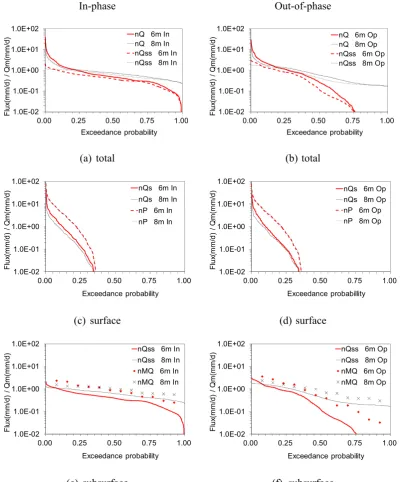
3.4 Sensitivity of the FDCs to soil depth
[image:9.595.97.496.71.558.2]2814 Y. Yokoo and M. Sivapalan: Towards reconstruction of the flow duration curve
1
1
In-phase Out-of-phase
1.0E-02 1.0E-01 1.0E+00 1.0E+01 1.0E+02
0.00 0.25 0.50 0.75 1.00
F
lu
x(
mm/
d
) /
Qm(
m
m/
d)
Exceedance probability nQ 6m In nQ 8m In nQss 6m In nQss 8m In
(a)
total
1.0E-02 1.0E-01 1.0E+00 1.0E+01 1.0E+02
0.00 0.25 0.50 0.75 1.00
Fl
ux
(m
m
/d)
/
Qm
(m
m
/d)
Exceedance probability nQ 6m Op nQ 8m Op nQss 6m Op nQss 8m Op
(b)
total
1.0E-02 1.0E-01 1.0E+00 1.0E+01 1.0E+02
0.00 0.25 0.50 0.75 1.00
Fl
ux
(m
m
/d
) /
Qm
(m
m/
d)
Exceedance probability nQs 6m In nQs 8m In nP 6m In nP 8m In
(c)
surface
1.0E-02 1.0E-01 1.0E+00 1.0E+01 1.0E+02
0.00 0.25 0.50 0.75 1.00
Fl
ux
(m
m
/d
) /
Qm
(m
m/
d)
Exceedance probabillity nQs 6m Op nQs 8m Op nP 6m Op nP 8m Op
(d)
surface
1.0E-02 1.0E-01 1.0E+00 1.0E+01 1.0E+02
0.00 0.25 0.50 0.75 1.00
Fl
ux
(m
m
/d)
/
Qm(
m
m
/d)
Exceedance probability nQss 6m In nQss 8m In nMQ 6m In nMQ 8m In
(e)
subsurface
1.0E-02 1.0E-01 1.0E+00 1.0E+01 1.0E+02
0.00 0.25 0.50 0.75 1.00
Fl
ux
(m
m/
d)
/
Qm
(m
m/
d)
Exceedance probability nQss 6m Op nQss 8m Op nMQ 6m Op nMQ 8m Op
(f)
subsurface
2
Figure 5
3
4
Fig. 5. Effect of soil depth for different climatic seasonality: (a), (b): Total flow FDC, (c), (d): surface flow FDC, (e), (f): subsurface flow FDC. (a), (c), (e): seasonal peaks ofP and PET are in phase, (b), (d), (f): seasonal peaks ofP and PET are of opposite phase. The “6 m” and “8 m” indicate soil depth for each experimental case. Qmis mean annual daily flow (mm d−1). “nMQ” refers to FDC associated with
the regime curve – ensemble averaged mean within-year daily variation normalized by mean annual daily flowQm. Default value of climate dryness isR= 0.5 (humid), soil type is silty loam, and topographic gradient is 0.006.
be seen in Fig. 5, four different cases are considered: two different soil depths (6 m and 8 m), and in-phase and out-of-phase seasonality. Figure 5a, c and e are for in-phase sea-sonality, and Fig. 5b, d and f are for out-of-phase seasonality. Figure 5c and d present the FDCs for surface runoff, whereas Fig. 5e and f present the FDCs for subsurface runoff.
[image:10.595.97.498.62.545.2]to generate partial saturated areas where ET is larger due to the moisture being more accessible to the influence of atmo-spheric demand while there is more chance for surface runoff to be generated over partial saturated areas as well. Note also that there is a deviation between the FDCs and SSFDCs at the upper tail. As before, this being a silty loam, the discrepancy is due to surface runoff contribution. This is also reflected in Fig. 5c and d; as before, the FDCs for surface runoff track PDC. However, since the surface runoff (especially by infil-tration excess) is a surface phenomenon, it is not affected by the depth of soil.
Figure 5e and f present a comparison between the SSFDCs and the FDCs derived from the regime curve. The results indicate that the SSFDCs generally track the FDCs gener-ated from the regime curve, especially when the soil is deep. However, there is a deviation towards the lower tail of the FDCs, and the deviation is larger in the case of out-of-phase seasonality. One can also see that the FDC generated from the regime curves also deviate in shallow soils from that for deep soils during low flows, which becomes even more sig-nificant whenP and PET are out of phase. Hence the estima-tion of SSFDC and FDC from mean monthly runoff (regime curve) would not be not so straightforward for basins with shallow soils. This is because shallow soil has smaller stor-age capacity and hence runoff is sensitive to precipitation and evapotranspiration. If precipitation stops, then ET would be-come more dominant during such dry periods as shown by Botter et al. (2007a,b). These observations lead us to the idea that ET may be playing a dominant role under dry conditions, as also highlighted in Figs. 3 and 4.
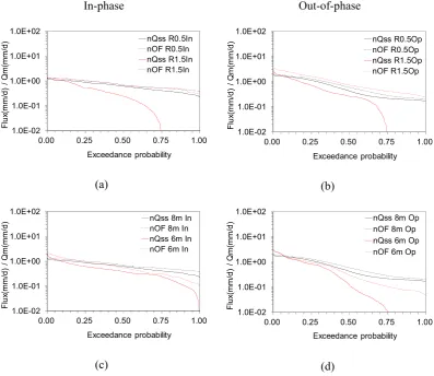
3.5 Possible reason for lower tail of the FDCs
Through Figs. 3 to 5, we have shown that the SSFDCs devi-ated from the FDCs generdevi-ated from the regime curve under arid climate and shallow soil, and it was difficult to repro-duce the shape of middle to lower flow parts of a FDC. In or-der to unor-derstand the possible reasons for the sharp dip of the FDC under arid climates and in shallow soils, we constructed the flow duration curves for outflows OF from the saturated zone along with the corresponding SSFDCs. In the model, subsurface flowQss is calculated as outflow OF minus the
product of saturated surface area fraction and ET from that saturated surface (which happens at the potential rate PET: indeed, when the product is higher than OF, thenQssis put
to zero and the product becomes equal to OF.) Therefore, any differences between the duration curves for OF andQss,
and the dip in the SSFDCs at low flows are potentially due to the ET from the saturated surface areas, and the temporal smoothing involved in constructing the regime curve.
The results are presented in Fig. 6. Panels a and b show the results for different climatic dryness and seasonality. Pan-els a and c are for in-phase seasonality, and panPan-els b and d are for out-of-phase seasonality. Default value of soil type is silty loam, soil depth is 8 m, the topographic gradient is 0.006,
and dryness index is 0.5. Through these results we assess the controls on the deviations by exploring the effects of cli-mate dryness in panels a and b, and the effects of soil depth in panels c and d. The results confirm that even when OF is non-zero during dry periods, the FDC for subsurface flows deviate downwards at low flow conditions, reaching zero for some 25 % of the time in arid catchments, which is caused by ET from partial saturated areas. We can also find that the slope of OF is high and the deviation is less during lowQss
periods ifP and PET are out of phase under arid climate, which reflects the seasonality of such climate where there is more chance of infiltration to the saturated zone during wet seasons to generate relatively sustainedQss. By comparing
the results in the panel c and d, we can notice that the devia-tion ofQssfrom OF is higher ifP and PET are out of phase
and/or soil depth is shallow. If a basin’s soil is shallow, water table appears close to the ground surface and the saturated surface area fraction increases. In addition, ET from the sat-urated surface becomes more dominant helping to expand the deviation whenP and PET are out of phase.
As shown here, the dip of a FDC under arid climates or shallow soils is potentially due to the dominance of ET from the saturated areas. In such basins, we would observe very little subsurface runoff (i.e. zero flows) for some period in a year, which causes the ephemeral runoff time series, making them different from the FDCs associated with mean monthly runoff (regime curve). Hence it would be difficult to estimate the FDC from a regime curve alone and it will be necessary to introduce a more sophisticated rainfall-runoff model to es-timate the shape of FDC. On the other hand, we would have more chance to reproduce the shape of a FDC from a regime curve if the basin is in a humid climate or has deep soils.
4 Discussion and conclusions
The flow duration curve represents the distillation of intra-annual variability of runoff, and presented in the frequency (probability) domain. It can be seen as a manifestation of the filtering by the catchment of within-year variability of pre-cipitation. Precipitation variability comprises variability at a range of scales, including random within-storm and between-storm variability as well as more systematic (e.g. seasonal) variability. In this paper we investigated the effects of cli-mate, soils, and topography on the shape of the FDC using a simple, physically based water balance model and synthetic rainfall data. The study focused on the fundamental ques-tions: what does the shape of the FDC represent, and what are its process controls?
2816 Y. Yokoo and M. Sivapalan: Towards reconstruction of the flow duration curve
1
1
In-phase Out-of-phase
1.0E-02 1.0E-01 1.0E+00 1.0E+01 1.0E+02
0.00 0.25 0.50 0.75 1.00
F
lu
x(
m
m/
d
) /
Qm
(m
m/d
)
Exceedance probability nQss R0.5In nOF R0.5In nQss R1.5In nOF R1.5In
(a)
1.0E-02 1.0E-01 1.0E+00 1.0E+01 1.0E+02
0.00 0.25 0.50 0.75 1.00
Fl
ux
(m
m/
d)
/
Q
m
(mm/
d)
Exceedance probability nQss R0.5Op nOF R0.5Op nQss R1.5Op nOF R1.5Op
(b)
1.0E-02 1.0E-01 1.0E+00 1.0E+01 1.0E+02
0.00 0.25 0.50 0.75 1.00
F
lu
x(
m
m/
d
) /
Qm
(m
m/d
)
Exceedance probability nQss 8m In nOF 8m In nQss 6m In nOF 6m In
(c)
1.0E-02 1.0E-01 1.0E+00 1.0E+01 1.0E+02
0.00 0.25 0.50 0.75 1.00
Fl
ux
(m
m/
d)
/
Q
m
(mm/
d)
Exceedance probability nQss 8m Op nOF 8m Op nQss 6m Op nOF 6m Op
(d)
2
3
Figure 6.
4
5
Fig. 6. Relationships between FDCs of the outflow OF and subsurface flowQssnormalized by mean annual daily flowQm: (a) seasonal peaks ofP and PET are both in phase but dryness indices are 0.5 and 1.5; (b) seasonal peaks ofP and PET are both of opposite phase and dryness indices are 0.5 and 1.5; (c) seasonal peaks ofP and PET are both in phase but soil depths are 6 m and 8 m; and (d) seasonal peaks of P and PET are both of opposite phase but soil depth is 6 m and 8 m. The difference betweenQmand OF is equal to the evapotranspiration from the saturated fraction of the ground surface. Default soil type, soil depth, topographic gradient, and dryness index are, respectively, silty loam, 8 m, 0.006, and 0.5.
drivers: precipitation and potential evaporation. The FDC is steeper when the seasonality ofP and PET are out of phase, in comparison to when they are in phase. In addition, the slope of the FDC is further enhanced in more permeable soils and in shallow soils. On the other hand, the effect of climate is such that with increasing aridity the flow becomes more ephemeral, with the result that the FDC tends to get cut off at low flows.
The results indicated that there is considerable potential to estimate the shape of a FDC in its middle and low flow parts from mean monthly runoff (regime curve) in basins under humid climate with relatively deep soils. However, in arid climates or catchments with shallow soils that tend to gen-erate ephemeral runoff, it is difficult to reproduce the shape of a FDC from the regime curve alone. To reproduce the shape of a FDC from a regime curve in circumstances where the effect of ET is strong (i.e. arid climate, shallow soils, out-of-phase seasonality), we need to explicitly consider a
correction to the middle and lower tail to account for the re-duction of subsurface drainage due to the effects of ET losses over the near-stream saturation areas. We would need a more sophisticated model including estimating ET losses, and in-corporating complex processes such as seasonal changes in leaf phenology.
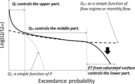
[image:12.595.97.495.64.408.2]1 1
Qscontrols the upper part.
Qsscontrols the middle part.
ET from saturated surface controls the lower part.
Log
(
Q
/
Qm
)
Exceedance probability Qs: a simple function of P
Qss: as a simple function of
flow regime or monthly flow.
2 3
4
Figure 7 5
[image:13.595.307.545.63.210.2]6
Fig. 7. Schematic illustrating the understanding gained through this simulation study regarding the shapes of the flow duration curve, including the controls on the different parts of the FDC.
surface phenomenon that can be captured using a nonlin-ear (threshold) filter. The dominant factors that control it are rainfall intensity patterns and soil (infiltration) character-istics, with very little influence of climate seasonality, soil depth or surface topography.
The SSFDC component, in most cases, is a much more smoothed component, with much of the event structure smoothed out. Instead, the shape of the SSFDC reflects the competition between seasonal variability of precipitation and potential evapotranspiration in the vadose zone, which gov-erns recharge to the water table, and then the filtering of the groundwater recharge flux by the dynamic aquifer through subsurface drainage. Previous work has explored the process controls on the recharge (Struthers et al., 2006; McGrath et al., 2007; Harman et al., 2011), and on shallow subsurface flow in hillslopes (Harman and Sivapalan, 2009).
Finally the dip of the flow duration curve at the lower tail arises due to the relatively higher ET from saturated surfaces, which happens in watersheds in arid climates or with lower storage capacity of soil. This is a feature that we could cap-ture with a quasi-2-D model that pays explicit attention to the water table profile and its intersection with the land surface. The main process controls are, therefore, topography, land-scape organization, depth to bedrock, and lateral saturated hydraulic conductivity.
On the basis of these considerations we are now in a posi-tion to formulate a conceptual framework for the reconstruc-tion of the flow durareconstruc-tion curve in ungauged basins. This is presented in Fig. 8. The conceptual framework comprises three components: (1) a simple nonlinear (threshold) filter model that captures surface infiltration losses, and in this way provide the transformation from PDC to SFDC; (2) estima-tion of the middle to lower flow parts of a FDC from a mean monthly runoff data in basins with perennial runoff. Mean monthly runoff is relatively easy to obtain from global runoff simulation model results or through extrapolation from mea-sured data in gauged basins. If the basin generates ephemeral
1 Qs
Qss
• P, PET
• Geophysical characteristics G
ET
Surface flow model
Subsurface flow model
Exceedance probability Log(Q/Qm)
ET model
P, PET G
P, PET G P
1
2
3
Figure 8. 4
5
Fig. 8. A conceptual model for reconstruction of the flow duration curves in ungauged basins, consisting of models of (i) partition-ing of precipitation into fast (surface) runoff and wettpartition-ing, which involves nonlinear (threshold filtering), (ii) the partitioning of the wetting into slow (subsurface) flow and evapotranspiration, which involves mainly linear filtering, and (iii) a correction to the FDC in flow situations due to evapotranspiration from saturated areas.
runoff, we would need to introduce a more complex two component model of the vadose zone coupled to a subsurface flow model, as a way to simulate realistic patterns of recharge to the water table and then its filtering in the shallow aquifer below; and (3) finally, we need a 2-D model in order to sim-ulate the dynamics of the near-stream saturated area so that we can estimate ET correction during low flow periods. Note that details for the nonlinear filter model of the above (1), a simple two component model of the vadose zone coulped to a shallow subsrface flow model of the above (2), and a 2-D model of the near stream saturated area of the above (3) must be constructed and parameterized for each basin; this forms part of our future work.
The insights gained into the shapes of FDCs, including their process controls, give us confidence that there is con-siderable potential for extrapolating the shapes of FDCs from daily precipitation data, monthly flow data, climatic dryness and storage capacity in gauged basins to ungauged basins, at least, in humid basins. Work being undertaken by the au-thors is aimed at implementing the conceptual framework developed here in over 200 catchments around the continen-tal United States, and using the data from these catchments to explore the spatial (regional) patterns of variations of the FDCs across the country, explain these patterns on the basis of available evidence on climate, soils and topography, and evaluate the power of the conceptual framework developed here to extrapolate FDCs from gauged basins to ungauged basins.
[image:13.595.50.283.65.209.2]2818 Y. Yokoo and M. Sivapalan: Towards reconstruction of the flow duration curve
1
1
1.E‐04 1.E‐03 1.E‐02 1.E‐01 1.E+00 1.E+01 1.E+02
0.00 0.25 0.50 0.75 1.00
Flu x( mm/ d) / Q m (mm/d )
Exceedance Probability
nP nQ nQs
nQss nMQ
2
(a)
MOPEX watershed #86, Salmon River at Salmon, Idaho, USA.
3
4
1.E‐03 1.E‐02 1.E‐01 1.E+00 1.E+01 1.E+02
0.00 0.25 0.50 0.75 1.00
Flu x( mm/ d) / Q m (mm/d )
Exceedance Probability
nQ nQs nQss
nMQ nP
5
(b)
MOPEX watershed #237, Nantahala River near Rainbow Springs, North Carolina, USA.
6
7
1.E‐04 1.E‐03 1.E‐02 1.E‐01 1.E+00 1.E+01 1.E+02
0.00 0.25 0.50 0.75 1.00
Flux( mm/d ) / Qm( mm/ d)
Exceedance Probaobility
nQs nQss nMQ
nP nQ
8
(c)
MOPEX watershed #323, Lochsa River near Lowell, Idaho, USA.
9
10
Figure 9.
11
1 11.E‐04 1.E‐03 1.E‐02 1.E‐01 1.E+00 1.E+01 1.E+02
0.00 0.25 0.50 0.75 1.00
Flu x( mm/ d) / Q m (mm/d )
Exceedance Probability
nP nQ nQs
nQss nMQ
2
(a) MOPEX watershed #86, Salmon River at Salmon, Idaho, USA. 3
4
1.E‐03 1.E‐02 1.E‐01 1.E+00 1.E+01 1.E+02
0.00 0.25 0.50 0.75 1.00
Flu x( mm/ d) / Q m (mm/d )
Exceedance Probability
nQ nQs nQss
nMQ nP
5
(b)MOPEX watershed #237, Nantahala River near Rainbow Springs, North Carolina, USA. 6
7
1.E‐04 1.E‐03 1.E‐02 1.E‐01 1.E+00 1.E+01 1.E+02
0.00 0.25 0.50 0.75 1.00
Flux( mm/d ) / Qm( mm/ d)
Exceedance Probaobility
nQs nQss nMQ
nP nQ
8
(c) MOPEX watershed #323, Lochsa River near Lowell, Idaho, USA. 9 10 Figure 9. 11 1 1
1.E‐04 1.E‐03 1.E‐02 1.E‐01 1.E+00 1.E+01 1.E+02
0.00 0.25 0.50 0.75 1.00
Flu x( mm/ d) / Q m (mm/d )
Exceedance Probability
nP nQ nQs
nQss nMQ
2
(a) MOPEX watershed #86, Salmon River at Salmon, Idaho, USA. 3
4
1.E‐03 1.E‐02 1.E‐01 1.E+00 1.E+01 1.E+02
0.00 0.25 0.50 0.75 1.00
Flu x( mm/ d) / Q m (mm/d )
Exceedance Probability
nQ nQs nQss
nMQ nP
5
(b)MOPEX watershed #237, Nantahala River near Rainbow Springs, North Carolina, USA. 6
7
1.E‐04 1.E‐03 1.E‐02 1.E‐01 1.E+00 1.E+01 1.E+02
0.00 0.25 0.50 0.75 1.00
Flux( mm/d ) / Qm( mm/ d)
Exceedance Probaobility
nQs nQss nMQ
nP nQ
8
(c) MOPEX watershed #323, Lochsa River near Lowell, Idaho, USA. 9
10
Figure 9.
11
Fig. 9. Three example applications of the concepts derived from this paper: Relationships among duration curves of precipitation (nP), total runoff (nQ), surface runoff (nQs), subsurface runoff (nQss), all at daily time scales and normalized by annual mean daily flow (Qm) along with mean monthly runoff (nMQ) at daily time scale normal-ized by annual mean daily flow (Qm). (a) data from MOPEX wa-tershed #86, Salmon River at Salmon, Idaho, (b) data from MOPEX watershed #237, Nantahala River near Rainbow Springs, North Car-olina, and (c) data from MOPEX watershed #323, Lochsa River near Lowell, Idaho.
estimated from the “regime curve” (mean monthly variation of total runoff). The surface and subsurface runoff compo-nents are estimated using a baseflow separation algorithm (Lyne and Hollick, 1979), which was previously summarized in Sivapalan et al. (2011). These results provide some con-firmation of the conclusions of this paper. In particular, one can see the close relationship between the PDCs and SFDCs, and the similarly strong relationships between the SSFDCs
and the FDCs associated with the regime curves. As shown above, we have confidence that the understandings gained on the process controls of FDCs, as outlined in the pro-posed framework for their reconstruction in ungauged basins would have considerable potential for broad applications in the future.
Acknowledgements. The first author is grateful for the financial support provided by the JSPS Research Fellowship for Young Scientists and the Grant-in-Aid for JSPS fellows that enabled the long-term collaboration that culminated in the publication of this paper. He also thanks the Grant-in-Aid for Young Scientists (B, 18760381, 21760381), Grant-in-Aid for Scientific Research (B, 22360192, PI: Prof. So Kazama at Tohoku University, Japan), research grant from Maeda Engineering Foundation, Environment Research and Technology Development Fund (S-8-1(4)) of the Ministry of the Environment, Japan, and the Science and Technol-ogy Research Partnership for Sustainable Development, JST-JICA, Japan, for providing additional support. The present study was also supported by “Wisdom of Water” (Suntory) Corporate Sponsored Research Program at the University of Tokyo, provided by the Sun-tory Corporation, Japan. The authors are also grateful to Taikan Oki of the University of Tokyo for his constructive comments on earlier drafts of this paper.
Edited by: P. Claps
References
Botter, G., Porporato, A., Daly, E., Rodriguez-Iturbe, I., and Ri-naldo, A.: Probabilistic characterization of base flows in river basins: Roles of soil, vegetation, and geomorphology, Water Re-sour. Res., 43, W06404, doi:10.1029/2006WR005397, 2007a. Botter, G., Peratoner, F., Porporato, A., Rodriguez-Iturbe, I., and
Rinaldo, A.: Signatures of large-scale soil moisture dynamics on streamflow statistics across U.S. Climate regimes, Water Resour. Res., 43, W11413, doi:10.1029/2007WR006162, 2007b. Botter, G., Porporato, A., Rodriguez-Iturbe, I., and
Ri-naldo, A.: Nonlinear storage-discharge relations and catch-ment streamflow regimes, Water Resour. Res., 45, W10427, doi:10.1029/2008WR007658, 2009.
Bras, R. L.: Hydrology – An Introduction to Hydrologic Science, Addison-Wesley- Longman, Reading, Mass., 1990.
Brooks, R. H. and Corey, A. T.: Properties of porous media af-fecting fluid flow, J. Irrig. Drain. Div. Am. Soc. Civ. Eng., IR2, 61–88, 1966.
Brutsaert, W.: Probability laws for pore-size distributions, Soil Sci., 101, 85–92, 1966.
Budyko, M. I.: Climate and Life, Academic Press, New York, 1974. Burt, T. P. and Swank, W. T.: Flow frequency responses to hardwood-to-grass conversion and subsequent succession, Hy-dol. Process., 6, 179–188, 1992.
Castellarin, A., Vogel, R. M., and Brath, A.: A stochastic index flow model of flow duration curves, Water Resour. Res., 40, W03104, doi:10.1029/2003WR002524, 2004a.
[image:14.595.74.261.61.467.2]Chow, V. T., Maidment, D. R., and Mays, L. W.: Applied Hydrol-ogy, McGraw-Hill, New York, 1988.
Farmer, D., Sivapalan, M., and Jothityangkoon, C.: Climate, soil, and vegetation controls upon the variability of water bal-ance in temperate and semi-arid landscapes: Downward ap-proach to water balance analysis, Water Resour. Res., 39, 1035, doi:10.1029/2001WR000328, 2003.
Harman, C. J. and Sivapalan, M.: Similarity framework to assess controls on subsurface flow dynamics in hillslopes, Water Re-sour. Res., 45, W01417, doi:10.1029/2008WR007067, 2009. Harman, C. J., Rao, P. S. C., Basu, N. B., McGrath, G. S., Kumar,
P., and Sivapalan, M.: Climate, soil and vegetation controls on the temporal variability of vadose zone transport, Water Resour. Res., doi:10.1029/2010WR010194, in press, 2011.
Holmes, M. G. R., Young, A. R., Gustard, A., and Grew, R.: A region of influence approach to predicting flow duration curves within ungauged catchments, Hydrol. Earth Syst. Sci., 6, 721– 731, doi:10.5194/hess-6-721-2002, 2002.
Huff, F. A.: Time distribution of rainfall in heavy storms, Water Resour. Res., 7, 1007–1018, 1967.
Iacobellis, V.: Probabilistic model for the estimation of T year flow duration curves, Water Resour. Res., 44, W02413, doi:10.1029/2006WR005400, 2008.
Kosugi, K.: Three-parameter lognormal distribution model for soil water retention, Water Resour. Res., 30, 891–901, 1994. Koutsoyiannis, D. and Foufoula-Georgiou, E.: A scaling model of
a storm hyetograph, Water Resour. Res., 29, 2345–2361, 1993. Lee, H., Zehe, E., and Sivapalan, M.: Predictions of rainfall-runoff
response and soil moisture dynamics in a microscale catchment using the CREW model, Hydrol. Earth Syst. Sci., 11, 819–849, doi:10.5194/hess-11-819-2007, 2007.
Li, H. and Sivapalan, M.: Effect of spatial heterogeneity of runoff generation mechanisms on the scaling behavior of event runoff responses in a natural river basin, Water Resour. Res., 47, W00H08, doi:10.1029/2010WR009712, 2011a.
Li, H., Sivapalan, M., and Tian, F.: Comparative diagnostic analysis of runoff generation processes in Oklahoma DMIP2 basins: The Blue River and the Illinois River, J. Hydrol., doi:10.1016/j.jhydrol.2010.08.005, in press, 2011b.
Lyne, V. and Hollick, M.: Stochastic time-variable rainfall-runoff. Proc. Hydrology and Water Resources Symposium, Perth, Inst. of Engrs. Australia, 89–92, 1979.
McGrath, G. S., Hinz, C., and Sivapalan, M.: Temporal dynamics of hydrological threshold events, Hydrol. Earth Syst. Sci., 11, 923–938, doi:10.5194/hess-11-923-2007, 2007.
Mohamoud, Y. M.: Prediction of daily flow duration curves and streamflow for ungauged catchments using regional flow duration curves, Hydrolog. Sci. J., 53, 706–724, doi:10.1623/hysj.53.4.706, 2008.
Muneepeerakul, R., Azaele, S., Botter, G., Rinaldo, A., and Rodriguez-Iturbe, I.: Daily streamflow analysis based on a two-scaled gamma pulse model, Water Resour. Res., 46, W11546, doi:10.1029/2010WR009286, 2010.
Musiake, K., Inokuti, S., and Takahashi, Y.: Dependence of low flow characteristics on basin geology in mountainous areas of Japan, IAHS Publ., 117, 147–156, 1975.
Reggiani, P., Sivapalan, M., and Hassanizadeh, S. M.: Conservation equations governing hillslope responses: Exploring the physical basis of water balance, Water Resour. Res., 36, 1845–1863, 2000. Robinson, J. S. and Sivapalan, M.: Temporal scale and hydrological regimes: Implications for flood frequency scaling, Water Resour. Res., 33, 2981–2999, 1997.
Sefton, C. E. M. and Howarth, S. M.: Relationships between dy-namic response characteristics and physical descriptors of catch-ments in England and wales, J. Hydrol., 211, 1–16, 1998. Sivapalan, M., Yaeger, M. A., Harman, C. J., Xu, X., and
Troch, P. A.: Functional model of water balance variability at the catchment scale: 1. Evidence of hydrologic similarity and space-time symmetry, Water Resour. Res., 47, W02522, doi:10.1029/2010WR009568, 2011.
Smakhtin, V. U.: Low flow hydrology: a review, J. Hydrol., 240, 147–186, 2001.
Struthers, I., Hinz, C., and Sivapalan, M.: A multiple wetting front gravitational infiltration and redistribution model for wa-ter balance applications, Wawa-ter Resour. Res., 42, W06406, doi:10.1029/2005WR004645, 2006.
Vogel, R. M. and Fennessey, N. M.: Flow-duration curves I: New in-terpretation and confidence intervals, J. Water Resour. Pl.-ASCE, 120(4), 485–504, 1994.
Vogel, R. M. and Fennessey, N. M.: Flow-duration curves II: A Re-view of applications in water resources planning, Water Resour. Bull., 31(6), 1029–1039, 1995.
Ward, R. C. and Robinson, M.: Principles of Hydrology, 3rd Edn., McGraw-Hill, Maidenhead, Berkshire, England, 1990.
Yilmaz, K. K., Gupta, H. V., and Wagener, T.: A process-based di-agnostic approach to model evaluation: Application to the NWS distributed hydrologic model, Water Resour. Res., 44, W09417, doi:10.1029/2007WR006716, 2008.
Yokoo, Y., Sivapalan, M., and Oki, T.: Investigating the roles of climate seasonality and landscape characteristics on mean annual and monthly water balances, J. Hydrol., 357, 255–269, 2008. Zehe, E., Lee, H., and Sivapalan, M.: Dynamical process upscaling
for deriving catchment scale state variables and constitutive re-lations for meso-scale process models, Hydrol. Earth Syst. Sci., 10, 981–996, doi:10.5194/hess-10-981-2006, 2006.