www.hydrol-earth-syst-sci.net/16/671/2012/ doi:10.5194/hess-16-671-2012
© Author(s) 2012. CC Attribution 3.0 License.
Hydrology and
Earth System
Sciences
Multiplicative cascade models for fine spatial downscaling
of rainfall: parameterization with rain gauge data
D. E. Rupp1, P. Licznar2, W. Adamowski3, and M. Le´sniewski3
1Oregon Climate Change Research Institute, College of Earth, Ocean and Atmospheric Sciences, Oregon State University, Corvallis, Oregon, USA
2Institute of Environment Protection Engineering, Wrocław University of Technology, Wrocław, Poland 3Municipal Water Supply and Sewerage Company in Warsaw, Warsaw, Poland
Correspondence to: D. E. Rupp ([email protected])
Received: 14 July 2011 – Published in Hydrol. Earth Syst. Sci. Discuss.: 25 July 2011 Revised: 21 November 2011 – Accepted: 21 February 2012 – Published: 6 March 2012
Abstract. Capturing the spatial distribution of high-intensity rainfall over short-time intervals is critical for accurately as-sessing the efficacy of urban stormwater drainage systems. In a stochastic simulation framework, one method of generating realistic rainfall fields is by multiplicative random cascade (MRC) models. Estimation of MRC model parameters has typically relied on radar imagery or, less frequently, rainfall fields interpolated from dense rain gauge networks. How-ever, such data are not always available. Furthermore, the literature is lacking estimation procedures for spatially in-complete datasets. Therefore, we proposed a simple method of calibrating an MRC model when only data from a mod-erately dense network of rain gauges is available, rather than from the full rainfall field. The number of gauges needs only be sufficient to adequately estimate the variance in the ra-tio of the rain rate at the rain gauges to the areal average rain rate across the entire spatial domain. In our example for Warsaw, Poland, we used 25 gauges over an area of approx-imately 1600 km2. MRC models calibrated using the pro-posed method were used to downscale 15-min rainfall rates from a 20 by 20 km area to the scale of the rain gauge capture area. Frequency distributions of observed and simulated 15-min rainfall at the gauge scale were very similar. Moreover, the spatial covariance structure of rainfall rates, as charac-terized by the semivariogram, was reproduced after allow-ing the probability density function of the random cascade generator to vary with spatial scale.
1 Introduction
Urban catchments, due to their diminished damping proper-ties relative to rural and natural catchments, are particularly responsive to bursts of local, high intensity rainfall. This makes characterization of the spatial distribution of rainfall at small time scales critical to evaluating the efficacy of urban stormwater drainage systems. Traditionally, design storms have been used to evaluate these systems in conjunction with rainfall-runoff and hydrodynamic models, but in recent years there has been a push towards stochastically downscaling long (e.g., multi-decadal) time series of coarse (e.g., daily) rainfall to higher resolution (e.g., minutes) with which to force models of stormwater drainage systems (e.g., Hingray and Ben Haha, 2005; Molnar and Burlando, 2005; Licznar et al., 2011a). Advantages of using long time series are that they allow for a statistical analysis of system performance and they eliminate the problem of defining the appropriate initial catchment water storage for a design storm (Hingray and Ben Haha, 2005). Furthermore, long time series of daily rainfall are already abundant and readily available, and time series of high-resolution rainfall with which to develop downscaling models are becoming more prevalent.
672 D. E. Rupp et al.: Parameterization of cascade models of rainfall fields
stochastic simulation approach. An alternative is to stochas-tically downscale the rainfall field as well as the time se-ries. For this purpose, a number of models for stochastically downscaling rainfall fields have been developed. Following Ferraris et al. (2003), most can be grouped into three gen-eral types: autoregressive models, point-process models that randomly position rainfall “cells”, and fractal and multifrac-tal cascade models. Additionally, there are hybrid models that combine features of these different approaches. For an overview of these various types, see Ferraris et al. (2003) and references therein. We focus on multifractal cascade models because, as noted by Veneziano et al. (2006), mul-tifractal models are simpler and have fewer parameters, and furthermore, though we do not consider these properties in this study, one can deduce the frequency distribution of rain-fall intensities and rainrain-fall extremes from their multi-fractal structure.
Parameter estimation for spatial downscaling models re-quires observations of the rainfall field. With multifractal cascade models, parameter estimation has mostly been done using radar-derived rainfall fields, though in a small num-ber of cases rainfall fields were generated by interpolating rain gauge data (Svensson et al., 1996; Jothityangkoon et al., 2000; Sharma et al., 2007). However, when the gauge den-sity is coarse relative to the final spatial resolution of interest, the interpolation methods will fail because they smooth out the fine-scale variability.
It is common for large metropolitan areas to have in excess of twenty rain gauges installed, whereas reliable fine scale radar-rainfall is less common (e.g., Thames Water, 2010). Even where radar imagery is available, there is value in es-timating model parameters directly from rain gauge data, given that accurate rainfall estimation from radar is complex and continues to be a focus of research (Krajewski and Smith, 2002; Pepler et al., 2011). Therefore, we propose a simple method of calibrating a multifractal cascade model for gen-erating rainfall fields of short-duration rainfall (e.g., 15 min) when information across the full field is not available, or specifically, when only data from a network of rain gauges is available. The number of gauges needs only be sufficient to adequately estimate the variance in the ratio of the rain rate at the rain gauges to the areal average rain rate across the entire spatial domain. We expect the particular number will depend on the degree of spatial variability across the domain of in-terest. We apply the calibration method to precipitation over Warsaw, Poland, and discuss error and bias in the estimation of the model parameters.
[image:2.595.311.547.69.377.2]In this study, we do not consider temporal evolution of the rainfall fields, which is required for a complete space-time downscaling model. Various cascade-based space-space-time models based on cascades have been proposed (e.g., Over and Gupta, 1996; Venugopal et al., 1999; Deidda, 2000; Jothityangkoon et al., 2000; Kang and Ramirez, 2010). Pa-rameterization of a space-time model will be a topic of a subsequent paper.
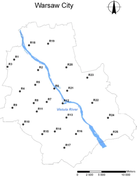
Fig. 1. Location of rain gauges used in study in Warsaw, Poland.
2 Data and methodology
2.1 Data
Rainfall data were collected from a network of 25 rain gauges distributed throughout Warsaw, Poland. The gauges were installed by Warsaw Waterworks in the fall of 2008 to bet-ter characbet-terize storm systems with the specific objective of modeling combined sewer- stormwater systems. Individual gauges were located to obtain best representative meteoro-logical observations in urban settings (Oke, 2006) and to have approximately constant gauge density over the entire city (Fig. 1). The gauges were connected to a single data acquisition system by means of general packet radio service (GPRS) modems. The data used in this study were recorded with a temporal resolution of 1 min and cover the period from the 38th week of year 2008 up to the 49th week of year 2010. For our analysis, data were included only when 21 or more gauges were operating.
D. E. Rupp et al.: Parameterization of cascade models of rainfall fields 673
precipitation was observed. However, at a 1-min resolution, the output signal was detectably more damped and broader than the input signal. As a consequence, rain was at times still being recorded for up to a few minutes after water was no longer being added to the gauge funnel. To reduce the relative error caused by this modulation of the signal, we aggregated the data to 15-min intervals.
Precipitation occurs in Warsaw as rain and snow and is generated during both frontal and convective storms. Scaling statistics may vary by precipitation type and storm type, so categorizing data by distinct meteorological processes can be revealing (Lovejoy and Schertzer, 1991; Harris et al., 1997). In Warsaw, snow is limited mainly to the months of Novem-ber through April, and averages 61 % of all precipitation in February (De¸bski, 1959). Though data on Warsaw storm types were not available to us, a recent analysis of precip-itation and circulation patterns at Krak´ow, Poland, 268 km south of Warsaw, showed daily precipitation events in the summer were nearly evenly divided between frontal rain-fall and non-frontal rainrain-fall (Twardosz et al., 2011). In win-ter, non-frontal rainfall was half as frequent as frontal rain-fall, while non-frontal snowfall was 50 % more frequent than frontal snowfall. The implication is that simply dividing the dataset by season would not be adequate, and we do not have sufficient information to categorize the Warsaw data by me-teorological process nor by precipitation type. Given that the focus of this paper is not the precise characterization of War-saw precipitation, grouping all the data does not detract from our primary purpose. From hereon, we make no distinction between rain and snow (as rain equivalent) and refer to all precipitation as “rainfall” to be consistent with the existing modeling literature.
2.2 Spatial downscaling model
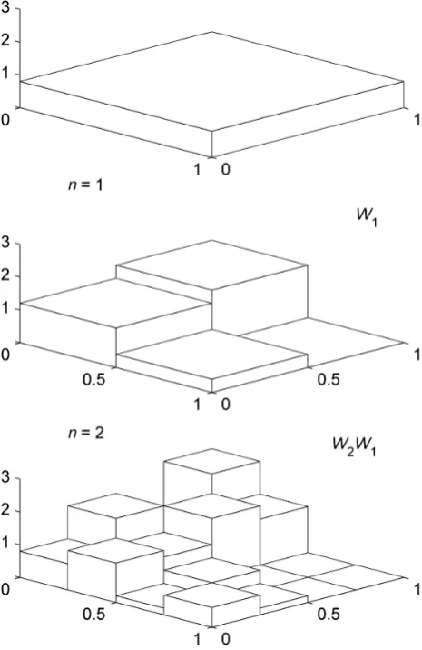
Our downscaling model is based on a discrete multiplica-tive random cascade (MRC). In the discrete MRC model of rainfall fields, the small-scale rainfall rate per unit area in a square cell1at thenth cascade level is given by
Rn 1n,k=R0 n Y
j=1
Wj,k (1)
where the area of1n is given by L20b−n. Here the large-scale rainfall rateR0is the rainfall amount over some interval of time per unit area over the host cell with areaL20. The constantb is the branching number, or number of sub-cells (in our case, 4) into which rainfall from a cell is partitioned at the next level in the cascade (Fig. 2). For each level, the index pair (j,k)represents the cell along the path to thenth level cell. The cells at then-th cascade level are indexed by1n,k,
[image:3.595.312.545.64.422.2]k= 1, 2, . . . , 4n (see Over and Gupta, 1996). The cascade weightWis a random variable with a prescribed distribution function, of which various types have been proposed in the context of rainfall (e.g., Schertzer and Lovejoy, 1987; Gupta
Fig. 2. Schematic of two-dimensional multiplicative cascade with
branching numberb= 4.
and Waymire, 1993; Over and Gupta, 1996; Deidda et al., 1999; Ahrens, 2003).
The weightW is generated as a random quantity with the following probability density:
P (W=0)=1−p (2)
P (W=p−1W+)=p (3)
whereP denotes probability,pis a parameter andW+are the non-zero (positive) weights (Over and Gupta, 1994). Equations (2) and (3) comprise the cascade generator: Eq. (2) generates the intermittency in the rainfall field (subareas of zero rainfall), while Eq. (3) generates the rainfall volumes greater than zero.
Samorodnitsky and Taqqu (1994). Properties of stable dis-tributions in the context of multifractal rainfall fields have been discussed by Schertzer and Lovejoy (1987), Lovejoy and Schertzer (1990), and Gupta and Waymire (1990, 1993), for example.
To ensure that the moments of W+ are finite, we set
β=−1 (Samorodnitsky and Taqqu, 1994). Furthermore, to conserve mass, on average, throughout the entire cascade process, we impose the condition that E[W+] =1. This means that
µ=σαsec(π α/2) (4)
(McCulloch, 1996), which leaves two free parameters α
and σ to describe the distribution. When α= 2, distribu-tion becomes normal with meanµand varianceσN2, where
σ=σN/
√
2.
2.3 Parameter estimation
Typically, estimation of spatial cascade model parameters relies on an analysis of the spatial scaling of the statisti-cal moments of the observed rainfall quantities (e.g., Over and Gupta, 1996; Deidda, 2000; Jothityangkoon et al., 2000; Pathirana and Herath, 2002; Sharma et al., 2007; Kang and Ramirez, 2010). Theq-th momentMat each spatial scaleλ
is calculated as
M(λn,q)=
X
k
Rn 1n,kq (5)
where the spatial scaleλn is given byLn/L0. Rainfall rates
Rn 1n,kat a particular scale λn are determined by aggre-gating observed rainfall into grids with cells of area1n. The relationship between the moments and scale is made through log-log plots ofM(λn,q)versusλn for various q. Linear-ity of the individual moments versus scale in log-log space implies either mono- or multifractality. The moment-scaling behavior of a fractal field has the form
M(λn,q)=(λ)τ (q) (6)
whereτ(q)versusq is either a line (monofractal) or a curve (multifractal). Finally, the parameters of the cascade gen-erator are estimated by fitting a distribution-dependent the-oretical function to the empirical relationship τ(q). For examples on how the moment-scaling estimation method would be applied to the MRC model such as the one de-scribed in Sect. 2.2, see Pathirana and Herath (2002) and Serinaldi (2010).
The above estimation method requires observed quanti-ties ofRn across a range of scalesλn. Unfortunately, we are hindered by a low gauge density (∼0.25 gauges km−2)
relative to a desirable grid cell density (on the order of 103 cells km−2, or a resolution of 30 by 30 m).
If we imposed fine resolution grids over our gauge net-work, very few cells would contain enough gauges to ad-equately estimate the areal-average rain rate for those cells.
Though we could use deterministic spatial interpolation tech-niques (e.g., Thiessen polygons) to estimate the rainfall ev-erywhere at every cell in the grid, this would likely result in a much too smooth rainfall surface.
Because of our inability to carry out a reliable analysis of moment scaling in space, we assumed a priori that there is power law scaling of the statistical moments. We based this assumption on previous observations of multifractality in rainfall fields for spatial scales under 30 km (e.g., Ku-mar and Georgiou, 1993a, b; Perica and Foufoula-Georgiou, 1996; Pathirana and Herath, 2002; Kang and Ramirez, 2010). Multifractality implies that realistic rain-fall fields could be reasonably reproduced, in a statistical sense, by a family of parsimonious multiplicative random cascade models.
As an alternative to moment-scaling analysis, we parame-terized our model using only the final product of the weights
W1throughWn, which we express by the variableY as
Yn 1n,k= n Y
j=1
Wj,k (7)
We consider the cases forY = 0 andY >0 separately. From Eq. (3), pj is the probability thatWj>0 along a path in anyj ofncascade levels. The probability thatY= 0 (which is to say that at least oneWj equals zero along the path down all n levels) can be calculated as 1 minus the probability thatWj is greater than zero in allnlevels. From the binomial distribution function (Ross, 1998) we obtain the solution for the probability thatY= 0:
P (Y=0)=1−
n Y
j=1
pj (8)
To help us determine the distribution ofY whenY >0, we defined the variableY+:
Yn+ 1n,k
=
n Y
j=1
Wj,k+ (9)
whereY+>0. Noting from Eq. (3) thatW=W+/p,Y can similarly be defined in terms ofW+as
Yn 1n,k= n Y
j=1
Wj,k+/pj
(10)
Combining Eqs. (9) and (10) and using the substitution
P (Y >0)=1−P (Y=0)yields the definition ofY+in terms ofY:
Y+=Y P (Y >0) (11)
For constant stability indexα, the log-stable distribution parameters forY+ can be easily determined from the log-stable parameters ofW+ because the product of log-stable variables is also log-stable. Let Y+=W1+W2+...Wn+ for
given by Wj+=exp(Xj), withXj∼SX(α,−1,σj,µj). If
Z=ln(Y+)=X1+X2+...+Xn, then Z is distributed as
Z∼SZ(α,−1,σZ,µZ), where
σZα=
n X
j=1
σjα (12)
and
µZ=
n X
j=1
µj (13)
forα6=1 (Samorodnitsky and Taqqu, 1994).
We estimated parameters for eight variations of vary-ing complexity of the MRC model described in Sect. 2.2. The simplest model used the log-normal distribution for
W+ with parameters that were scale-invariant and rainfall-independent, whereas the most complex used the stable dis-tribution with parameters that depended on both scale and rainfall. Each model is summarized below:
1. SIσ/RIσ/LN: the σ parameter of the cascade genera-tor was scale invariant (SIσ) andW+was log-normally (LN) distributed and independent of rainfall intensity (RIσ).
2. SIσ/RIσ/LS: the σ parameter of the cascade genera-tor was scale invariant andW+ had a log-stable (LS) distribution and was independent of rainfall intensity. 3. SIσ/RDσ/LN: the σ parameter of the cascade
gen-erator was scale invariant and W+ was log-normally distributed and dependent on rainfall intensity (RDσ). 4. SIσ/RDσ/LS: theσ parameter of the cascade generator
was scale invariant andW+had a log-stable distribution that was dependent on rainfall intensity.
5. SDσ/RIσ/LN: theσparameter of the cascade generator was scale dependent (SD) and W+ was log-normally distributed and independent of rainfall intensity. 6. SDσ/RIσ/LS: theσ parameter of the cascade generator
was scale dependent andW+had a log-stable distribu-tion and was independent of rainfall intensity.
7. SDσ/RDσ/LN: theσ parameter of the cascade gener-ator was scale dependent and W+ was log-normally distributed and dependent on rainfall intensity.
8. SDσ/RDσ/LS: the scale parameter σ of the cascade generator was scale dependent andW+had a log-stable distribution and was dependent on rainfall intensity. For those models whereσ was scale invariant,σwas solved for uniquely in terms ofσZby inverting Eq. (12):
σ=n−1/ασZ (14)
When σ was scale dependent, σ varied as the following function of the length scaleλ=L/L0:
σα(λ)=σ1αλγ (15)
whereγ is a constant andσ1is the value ofσ atλ= 1. For
γ >0, as the scaleλdecreases the variance ofW+decreases, which places it in the family of “bounded” cascade models (Marshak et al., 1994). Combining Eqs. (12) and (15) and using the substitutionλ=(1/2)j−1,σ1α can be solved for in terms ofσZ:
σ1α= 1−2 −γ
1−2−nγσ α
Z (16)
forγ >0
In all eight models, the intermittency parameter was determined fromP (Y >0):
p=[P (Y >0)]1/n (17)
Because it has been observed that spatial cascade parame-ters, and the intermittency parameter in particular, depend on large-scale rainfall (Over and Gupta, 1994, 1996; Dei-dda, 2000; Jothityangkoon et al., 2000; Pathirana and Herath, 2002; Deidda et al., 2004, 2006; Sharma et al., 2007), we al-lowed some of the parameters of the cascade generator to vary with the large-scale rainfall depth R0. While it has been argued that for both space (Veneziano et al., 2006) and time (Veneziano et al., 2006; Rupp et al., 2009; Serinaldi, 2010) the parameters should vary with rainfall intensity at each scale (not just the largest scale), our dataset did not permit us to adequately examine rainfall dependency across scales, therefore we restricted the dependency to the large-scale rainfall only.
In all eight models, we allowed the intermittency parame-ter to depend on large-scale rainfall by varyingP (Y >0)in Eq. (17) withR0as
P (Y >0)=1
2
1+erf
ln(R
0)−m
√
2s2
(18) where erf is the error function with parametersmands(Rupp et al., 2009). In four of the models, the scale parameterσ
was varied with rainfall by relatingσZin Eqs. (14) and (16) toR0as
σZ=c+f (R0) (19)
wheref ()is an arbitrary function and cis a constant. We used cubic splines to determinef ().
Observations of rainfall at gauges were used to estimate values of Y, Y+, and P (Y >0). Combining Eqs. (1) and (7) yieldsYn=Rn/R0, from which we see that an estimate of Y from observations ofR at a given rain gauge can be calculated as
ˆ Yi,k=
Ri,k
R0,i
whereYˆ is the estimate ofY ,i= 1, 2, . . . ,N
obsindexes the
i-th observation in time, andk= 1, 2, . . . , Ngauges indexes the rain gauge. The areal average rainfall R0,i at the ref-erence lengthL0 was approximated by taking the mean of the rainfall measured over allNgaugesat timei. To estimate
P (Y=0), we used
ˆ
Pi(Y >0)=(number of gauges with non−zero rain)i/Ngauges (21) Finally,Y+was estimated with
ˆ
Yi,k+= ˆYi,kPˆi(Y >0) (22)
BecauseY+is bounded by zero and positive infinity, whereas the upper limit toYˆ+isNgauges, the distribution ofYˆ+is only approximately equal to the distribution ofY+. This limita-tion, plus instrument error at very low and very high rain-fall intensities, introduces a bias into the estimation ofσZ. For now, we simply accept this bias as a shortcoming of the estimation procedure, though we discuss it further in Sect. 3. Free software packages for estimating the parameters of the stable distribution are rare, and we found none that suited our particular needs. For this reason, we used a simple procedure to estimateαZ andσZ from the “observed” val-ues lnYˆ+. An optimization algorithm minimized the sum of squared differences between the following observed and theoretical quantiles: 0.05, 0.1, 0.25, 0.5, 0.75, 0.9, and 0.95. For the normal distribution, we used the maximum likelihood method.
Note that except for at the largest spatial scale, we did not areally average the precipitation data. We also did not con-sider the particular location in space of the observed rain-fall. Both of these characteristics distinguish our study from others. However, we did use the number of cascade lev-elsn that brought us to the scale of the rain gauge itself. Given that the rain gauges have a diameter of approximately 0.15 m, and that the spatial extent of our rain gauge network corresponds to approximatelyL0= 20 000 m, approximately
n= 17 cascade levels are needed. 2.4 Model evaluation
[image:6.595.303.549.90.563.2]Direct comparison of the stochastically downscaled data to the observed rainfall requires disaggregation down to the capture area of the rain gauge throughn= 17 cascades levels, which would result in a grid with over 17×109cells. This would be impractical, especially given that very many such spatial fields would be generated for time increments of as little as 15 min. Instead of generating complete rainfall fields at the spatial resolution of a rain gauge, we followed the cas-cade process down a subset of the total number of possible paths down the cascade. Along a path at each subdivision, we randomly chose 1 of the 4 cells (with equal weight given to each cell), and tracked the position (x,y) of the cell for each of then= 17 cascade levels. In total, we followed 240 paths
Fig. 3. Probability of zero rain at a rain gauge, or equivalently,
P (Y= 0), against large-scale areal-averaged rainfall rate R0 for R0>0. (a):P (Y= 0) as estimated from the observed rainfall (light
D
e
n
s
it
y
-5 -4 -3 -2 -1 0 1 2
0
0
.8
1
.8
2
.8
3
.8
4
.8
2e-04 mm
-5 -4 -3 -2 -1 0 1 2
0
0
.8
1
.6
2
.4
3
.2
4
4e-04 mm
-5 -4 -3 -2 -1 0 1 2
0
0
.6
1
.4
2
2
.6
3
.4
4
0.001 mm
D
e
n
s
it
y
-5 -4 -3 -2 -1 0 1 2
0
0
.4
1
1
.4
2 0.0025 mm
-5 -4 -3 -2 -1 0 1 2
0
0
.2
0
.4
0
.6
0
.8 0.0063 mm
-5 -4 -3 -2 -1 0 1 2
0
0
.2
0
.4
0
.6 0.0158 mm
D
e
n
s
it
y
-5 -4 -3 -2 -1 0 1 2
0
0
.2
0
.4
0
.6 0.0398 mm
-5 -4 -3 -2 -1 0 1 2
0
0
.2
0
.4
0
.6
0
.8 0.1 mm
-5 -4 -3 -2 -1 0 1 2
0
0
.2
0
.4
0
.6
0
.8
1
0.2512 mm
ln(Y+)
D
e
n
s
it
y
-5 -4 -3 -2 -1 0 1 2
0
0
.2
0
.4
0
.6
0
.8 0.631 mm
ln(Y+)
-5 -4 -3 -2 -1 0 1 2
0
0
.2
0
.4
0
.6 1.5849 mm
ln(Y+)
-5 -4 -3 -2 -1 0 1 2
0
0
.2
0
.4
3.9811 mm
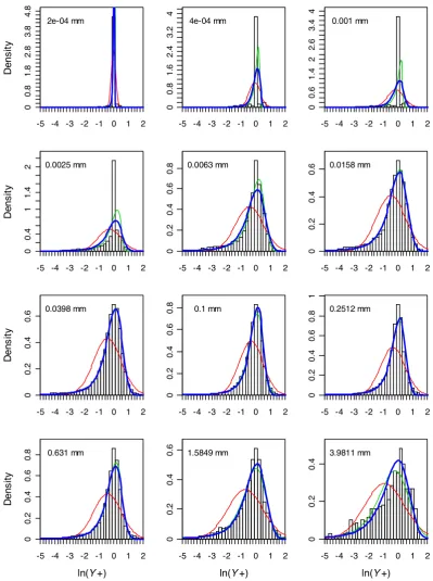
Fig. 4. Empirical density (bars) of lnY+and densities of the fitted stable distribution withαZas a fitting parameter (thin green line), withαZ
fixed at 1.47 (heavy blue line) and withαZfixed at 2 (thin red line). Distributions are shown for various large-scale areal-averaged rainfall
ratesR0(as mm per 15-min) forR0>0. The rainfall value shown in each plot is the midpoint of the range of log-transformed rainfall used
[image:7.595.97.497.93.629.2]per min increment. We used Eq. (1) to calculate the 15-min rainfall amounts at each of these 240 locations, which served as our representative “gauges”.
To further reduce the computational burden, downscaling was done on a sub-sample of all 18 723 15-min time steps whereR0>0. We selected 2000 time steps such that the cumulative distribution function (CDF) of the sub-sampled
Rnwas similar to the CDF of the full record.
The spatial structures of the observed and simulated 15-min rainfall were compared using semivariograms of log(Rn)forRn≥0.001 mm (15 min)−1(the minimum rain-fall amount recorded). The spatial structure of the intermit-tency was examined with semivariograms of presence (1) and absence (0) of rain.
In addition to the spatial structure, we assessed the abil-ity of the models to reproduce the cumulative distribution frequency (CDF) of 15-min rainfall forRn>0.
To examine the bias in the estimation method, we ran addi-tional simulations as described above in which we recorded the rainfall at 24 locations and used all 18 723 15-min time steps. From both the 240- and 24-gauge datasets, we esti-mated the model parametersm,s, andαZandσZusing the methodology described in Sect. 2.3.
3 Results and discussion
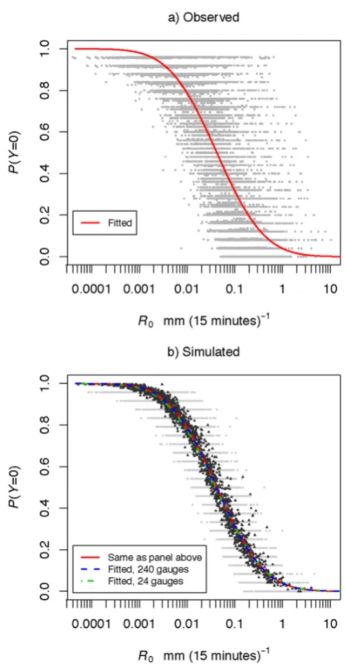
The proportion of gauges with zero rain in a 15-min period,
P (Y=0), was found to be strongly dependent on the large-scale rainfall rateR0(Fig. 3a). Consistent with many other studies (e.g., Over and Gupta, 1994, 1996; Jothityangkoon et al., 2000; Pathirana and Herath, 2002; Sharma et al., 2007), the sparseness of the rain field was much greater whenR0 was low, while at high rainfall rates the tendency was for it to be raining everywhere. The sigmoidal shape of Eq. (18) appears suitable for simulating the rainfall intermittency, as it allows forP (Y=0)to go to 1 asR0goes to 0, and to go to 0 asR0goes to+∞.
The empirical histograms of lnY+were rightward skewed, thus more similar to a log-stable density withβ=−1 than to a log-normal distribution (Fig. 4). At progressively lower val-ues ofR0, e.g., <∼0.01 mm (15 min)−1, the empirical his-tograms were progressively more dominated by lnY+=0, such that neither the log-stable nor the log-normal densities matched the observations. It is clear that by fitting theoreti-cal distributions to lnY+at low values ofR0, we are merely fitting to a data artifact and not to true rainfall behavior.
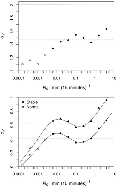
The value of the stable distribution parameterαZshowed a general increasing trend with increasingR0(Fig. 5). How-ever, whenαZ was fixed at a constant value of 1.47, the fits of the log-stable distributions were only marginally degraded (Fig. 4). This was fortunate because it allowed us to keep
αZas a constant parameter and only have to vary the scale parameterσZwith large-scale rainfall. The particular value ofαZ= 1.47 is the averageαZ using all values of lnYˆ+ for
R0 mm (15 minutes)!1
"Z
0.0001 0.001 0.01 0.1 1 10
1
1.2
1.4
1.6
1.8
2
R0 mm (15 minutes)!1
#Z
0.0001 0.001 0.01 0.1 1 10
0
0.2
0.4
0.6
0.8
1
Stable Normal
Fig. 5. Estimated stable distribution parameters αZ and σZ for Z=lnY+against large-scale areal-averaged rainfall ratesR0 for R0>0. The open symbols indicate where estimation was clearly
affected by artifacts arising from data precision. In the upper panel, the dashed line shows the estimate of αZ using all data
forR0≥0.004 mm (15-min)−1and the dotted line isσZ= 2 (the
normal distribution). In the lower panel, values of σZ assume
constantαZ= 1.47 andαZ= 2 for the stable and normal
distribu-tions, respectively. The solid curves are fitted cubic spline func-tions. The dashed and dotted horizontal lines indicate the values ofσZaveraged over allR0≥0.004 mm for the stable and normal
distribution, respectively.
R0≥0.004 mm. The threshold of 0.004 mm was selected because below this value the empirical distributions appeared to be strongly influenced by data precision (Fig. 4).
The dependency ofσZonR0was complex (Fig. 5), though cubic splines with no more than 6 knots reproduced the em-pirical relationship ofσZwithR0well. The relationship was similar in form for both the log-stable (αZ= 1.47) and log-normal (αZ= 2) distributions (Fig. 5). The range ofσZacross
[image:8.595.309.544.63.438.2]D. E. Rupp et al.: Parameterization of cascade models of rainfall fields 679
Log-normal - RI
S
e
m
iv
a
ri
a
n
c
e
Obs 0 0.4 0.8 1.2
0 5 10 15 20 25
0
0
.2
0
.4
0
.6
0
.8
1
Log-normal - RD
Obs 0 0.4 0.8 1.2
0 5 10 15 20 25
0
0
.2
0
.4
0
.6
0
.8
1
Log-stable - RI
Distance (km)
S
e
m
iv
a
ri
a
n
c
e
Obs 0 0.4 0.8 1.2
0 5 10 15 20 25
0
0
.2
0
.4
0
.6
0
.8
1
Log-stable - RD
Distance (km)
Obs 0 0.4 0.8 1.2
0 5 10 15 20 25
0
0
.2
0
.4
0
.6
0
.8
1
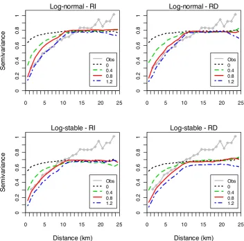
Fig. 6. Semivariogram of log-transformed rainfall ratesR >0.001 mm (15-min)−1from rain gauges (gray heavy line and solid circles) and from simulations (colored lines) using log-normal and log-stable distributions, rainfall independent (RI)σ, rainfall dependent (RD)σ, scale independentσ(γ= 0) and scale dependentσ(γ= 0.4, 0.8, and 1.2).
R0are suspect, as we have already determined the empirical distributions to be unreliable.
If we ignoreσZ for R0<0.01 mm (15-min)−1, the pat-tern in Fig. 5 (lower panel) implies a smoother field at in-termediate rainfall rates of about 0.1 mm (15-min)−1 and a more variable field at lower and higher rates. This trend toward higher variability at the highest rainfall rates could be the result of localized, high-intensity rainfall generated from strong convective storm cells. This trend is not evi-dent in the studies of Over and Gupta (1996), Jothityangkoon et al. (2000), Pathirana and Herath (2002), Veneziano et al. (2006), or Sharma et al. (2007), who only observed the scale parameter (i.e., variance) to decrease with increas-ing R0 from intermediate to high R0. The difference be-tween our and previous results may be due to differences in scales between studies: Jothityangkoon et al. (2000) and Sharma et al. (2007) analyzed daily rainfall, while Over and Gupta (1996), Veneziano et al. (2006) and Pathirana and Herath (2002) analyzed radar scans with resolutions ranging between 1 to 5 km.
The semivariogram of the observed rainfall rates shows covariability in rainfall intensity increasing strongly with in-creasing separation distance (Fig. 6). In contrast, all the scale-invariant models produced rainfall fields that showed little change in correlation with separation, though proximal rain was slightly more similar than distant rain. When the scale parameter σ as allowed to decrease with decreasing scale via Eq. (15), however, the general variogram pattern of the observed rainfall could be reproduced for separation distances of less than about 10 km by using a value ofγ ∼
[image:9.595.121.474.59.406.2]Distance (km)
S
em
iv
a
ri
a
nc
e
Obs 0 0.4 0.8 1.2
0 5 10 15 20 25
0
0
.0
4
0
.0
8
0
.1
[image:10.595.52.280.60.263.2]2
Fig. 7. Semivariogram of 15-min rainfall presence/absence from
rain gauge data (heavy gray line and solid circles) and from sim-ulations (colored lines) using Models SIσ/RIσ/LN (γ= 0) and SDσ/RIσ/LN withγ= 0.4, 0.8, and 1.2.
process might remove this artifact; we return to this point briefly at the end of this section.
The semivariogram of the presence/absence observations shows that if it is raining (or not raining) at one location, it is more likely to be raining (or not raining) nearby than it is further away (Fig. 7). The simulated rainfall fields have this property as well (at least below the 10 km sep-aration distance), but not to the degree of the observed rainfall field. Figure 7 gives semivariograms of the simu-lated presence/absence data using Models SIσ/RIσ/LN and SDσ/RIσ/LN only: semivariograms from all eight models were similar because the models are identical in how they simulate intermittency.
As mentioned above, the discrete cascade process pro-duces a blocky pattern, which will have some influence of the semivariogram. To generate patterns that are more re-alistic, a filter may be applied to the discretely generated field (Schertzer and Lovejoy, 1987; Menabde et al., 1997; Watson, R. J. and Hodges, D. D., 2005), or one may opt for a in-scale cascade, such as the continuous-in-scale universal multifractal (UM) model (Schertzer and Lovejoy, 1987; Lovejoy and Schertzer, 2010a, b). How a filter would affect the parameter estimation procedure pre-sented here, and how the parameter estimation would be done in the framework of the UM model, are topics of future study. Over most of the range ofR, the log-normal models repro-duced well the observed CDF of rainfall rates (Fig. 8). How-ever, the simulated CDFs using the log-normal models di-verged from the observed CDF below 0.02 mm (15-min)−1. The rainfall-dependent (RD) models performed slightly bet-ter than the rainfall-independent (RI) models up to the very highest rainfall intensities. Above about 15 mm (15-min)−1,
R0 mm (15 minutes)!1
Prob(
R
<
r
)
0.001 0.01 0.1 1 10 100
1e−05 1e−04 0.001 0.01 0.1 0.25 0.5 0.75 0.9 0.99 0.999 0.9999 0.99999
[image:10.595.313.541.61.261.2]Observed, subset Observed, all RI & SI RI & SD (0.8) RD & SI RD & SD (0.8)
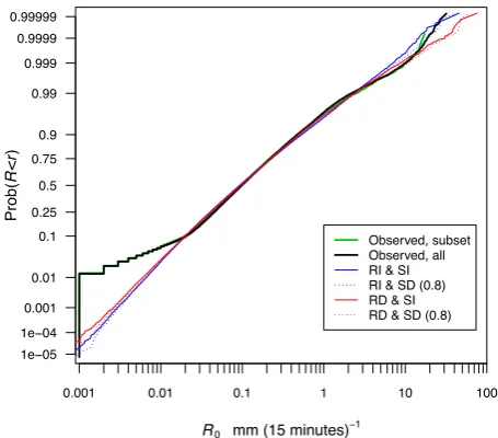
Fig. 8. Cumulative distribution function (CDF) of non-zero
rafall rates from all observations, of the subset of 2000 15-min in-tervals used to initialize the large-scale rainfallR0 for the simu-lations, and of the simulations. Simulated rainfall was generated using log-normal Models SIσ/RIσ/LN, SDσ/RIσ/LN withγ= 0.8, SIσ/RDσ/LN, and SDσ/RDσ/LN withγ= 0.8.
the rainfall-dependent models overestimated the rainfall in-tensity at a given probability of occurrence by roughly a factor of two.
The log-stable models did better than the log-normal mod-els at reproducing the overall shape of the observed CDF (Fig. 9), including matching the curvature forR <0.02 mm (15-min)−1. The log-stable models also mimicked the up-ward curvature of the observed CDF for the highest val-ues ofR, though they did under-predict the probabilities of these extreme events. Making the scale parameter rainfall-dependent resulted in an improved CDF, though at the high-est intensities these models still underhigh-estimated the rainfall intensity at a given probability of occurrence by as much as a factor of two.
R0 mm (15 minutes)! 1
Prob(
R
<
r
)
0.001 0.01 0.1 1 10 100
1e−05 1e−04 0.001 0.01 0.1 0.25 0.5 0.75 0.9 0.99 0.999 0.9999 0.99999
[image:11.595.319.534.60.403.2]Observed, subset Observed, all RI & SI RI & SD (0.8) RD & SI RD & SD (0.8)
Fig. 9. Cumulative distribution function (CDF) of non-zero
rafall rates from all observations, of the subset of 2000 15-min in-tervals used to initialize the large-scale rainfallR0 for the
simu-lations, and of the simulations. Simulated rainfall was generated using log-stable Models SIσ/RIσ/LS, SDσ/RIσ/LS withγ= 0.8, SIσ/RDσ/LS, and SDσ/RDσ/LS withγ= 0.8.
Additional bias, as already introduced in Sect. 2.3, arises from sampling the full rainfall field with a limited num-ber of gauges. In the case of rain intermittency, sampling introduced error into the estimation of P (Y=0), as seen from the deviations of the estimated from the assumed val-ues ofP (Y=0)in Fig. 3b. However, bias in the estima-tion of the intermittency parameters m and s in Eq. (18) was very small (Fig. 3b). From the observations, we esti-mated the pair (m,s)to equal (−3.170, 1.804), while from the simulations using all the scale invariant models, (m,s)
averaged (−3.177, 1.793) and (3.211, 1.809) with 240 and 24 gauges, respectively.
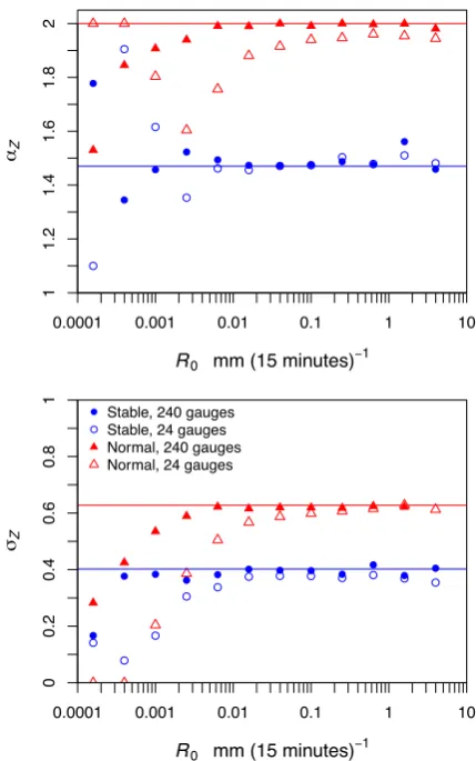
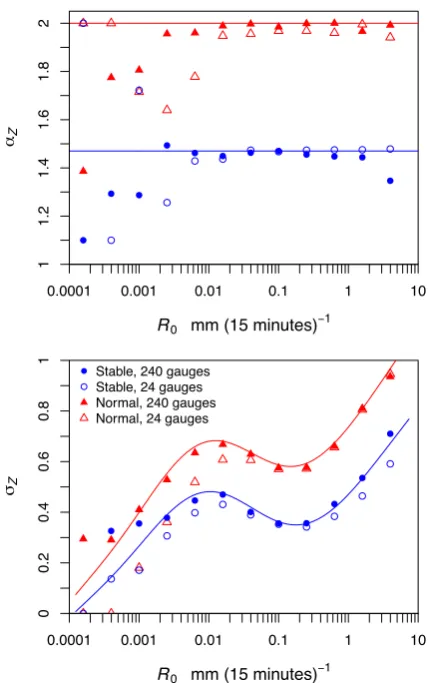
The bias effect of sample size was more prominent for the stable distribution parameters. The simulations using the scale-independent and rainfall-independent models provide a good illustration of this effect because the model param-eters never varied. In general, when the sample consisted of 240 gauges, the estimation procedure accurately retrieved the assumed values of αZ andσZ (Fig. 10). However, at progressively lowerR0, the parameter values were increas-ingly underestimated, and at the lowest values ofR0, there were simply to few observations to reliably fit the theoretical distributions to the data. Excluding lowR0, when the sample consisted of 24 gauges, there was no notable bias inαZwhen the rainfall came from a log-stable model, but there was a slight underestimationαZwhen the rainfall came from a log-normal model. On consequence is that one might choose a log-stable model when in fact the simpler log-normal is more appropriate. Even so, given the high values ofαZ(>1.9) es-timated here, use of the more complicated log-stable model
R0 mm (15 minutes)!1 "Z
0.0001 0.001 0.01 0.1 1 10
1
1.2
1.4
1.6
1.8
2
R0 mm (15 minutes)!1 #Z
0.0001 0.001 0.01 0.1 1 10
0
0.2
0.4
0.6
0.8
1
Stable, 240 gauges Stable, 24 gauges Normal, 240 gauges Normal, 24 gauges
Fig. 10. Stable distribution parametersαZandσZforZ=lnY+
against large-scale areal-averaged rainfall ratesR0forR0>0 as
es-timated from simulated rainfall using the rainfall-independent mod-els SIσ/RIσ/LS (log-stable) and SIσ/RIσ/LN (log-normal). The blue and red horizontal lines show the assumed values of αZ
(upper panel) and σZ (lower panel) for models SIσ/RIσ/ST and
SIσ/RIσ/LN, respectively. The solid symbols show the parameter values estimated using 240 “gauges”, represented by 240 grid cells in finest resolution field (approximately 15 cm×15 cm). The open symbols show the parameter values estimated using 24 such gauges.
would hardly be justified. Again, when using 24 gauges, there was a slight underestimation in σZ and it would ap-pear that this bias would increase with decreasing sample size. We obtained similar results using the rainfall-dependent models (Fig. 11).
It is clear from Figs. 10 and 11 that estimation accu-racy deteriorates at rainfall rates below about 0.01 mm (15-min)−1 with 24 gauges and below about 0.001 mm (15-min)−1for 240 gauges. The decrease inσZwith decreasing
[image:11.595.54.280.62.261.2]R0 mm (15 minutes)!1
"Z
0.0001 0.001 0.01 0.1 1 10
1
1.2
1.4
1.6
1.8
2
R0 mm (15 minutes)!1
#Z
0.0001 0.001 0.01 0.1 1 10
0
0.2
0.4
0.6
0.8
1
[image:12.595.59.274.59.401.2]Stable, 240 gauges Stable, 24 gauges Normal, 240 gauges Normal, 24 gauges
Fig. 11. Stable distribution parametersαZ andσZforZ=lnY+
against large-scale areal-averaged rainfall ratesR0forR0>0 as
es-timated from simulated rainfall using the rainfall-dependent mod-els SIσ/RDσ/LS (log-stable) and SIσ/RDσ/LN (log-normal). The blue and red horizontal lines show the assumed values ofαZ
(up-per panel) and σZ (lower panel) for models SIσ/RDσ/ST and
SIσ/RDσ/LN, respectively. The solid symbols show the parame-ter values estimated using 240 “gauges”, represented by 240 grid cells in finest resolution field (approximately 15 cm×15 cm). The open symbols show the parameter values estimated using 24 such gauges.
A variety of procedures could be used to partly account for the bias. One is to iteratively adjust the model pa-rameters until the estimated papa-rameters from the simulated dataset are nearly the same as those from the observed dataset (Veneziano et al., 2006). Another procedure is to exclude some data while estimating parameters. For example, in our study we left out data whereR0<0.004 mm (15-min)−1 when estimating αZ and when estimatingσZ for the case where σZ was assumed to be independent of R0. How-ever, this excluded only a relatively small amount of data and thus did not greatly affect the values ofαZand ofσZ inde-pendent ofR0. Furthermore, if the objective were to have rainfall-dependent parameters, excluding the low intensity
data would provide no guidance as to which parameter values to actually apply at these low rainfall intensities. In another example of censuring data, Licznar et al. (2011a) simply eliminated what would be analogous in our study to all val-ues ofY+= 1 from the empirical frequency distribution, un-der the assumption that most of these values were artifactual. A third procedure to deal specifically with recording preci-sion is to add random noise to the rainfall observations, with the intent of replacing the information lost by round-off error and thus removing the discretization that leads to an excess of certain values ofW+(orY+)(Licznar et al., 2011b).
Bias-correcting procedures such as those above should be explored, and we expect that they would improve the fits of frequency distributions. We know, for example, that both data precision and the finite number of gauges serve to de-crease the estimated value of the scale parameterσZ, in the former case by generating an overabundance ofYˆ+= 1 and in the latter case by imposing a maximum value toYˆ+ of
Ngauges. A bias-correcting procedure that led to an increase in the value of the log-stable parameterσZwould produce more extreme events, resulting in a CDF more like the observed one in Fig. 9. It would also increase the semivariance overall, which was generally underpredicted by the log-stable models (Fig. 6, lower panel).
Lastly, we have assumed stationarity in the rainfall field, though there may be long-term spatial patterns across the Warsaw metropolitan area. With our short record length (less than 3 yr) it would be difficult detect any but very clear and strong large-scale patterns, which we did not see. Should continuing observations reveal deterministic patterns in the spatial distribution of rainfall, we could account for these within the MRC framework. Examples of how this might be done using a deterministic field of weights that are ap-plied to the cascade generator are given by Jothityangkoon et al. (2000) and Pathirana and Herath (2002).
4 Conclusions
We have presented and evaluated a method for estimating the parameters of a multiplicative random cascade model for downscaling rainfall fields when observations of the full fields are not available either from radar imagery or from interpolation of very dense rain gauge network data. The estimation procedure still relies on rain gauge data, but the density of the network need only be such that (1) the rain-fall rate over a given time interval averaged over the entire spatial domain can be reasonably approximated by averag-ing the rainfall rate from all the gauges, (2) the number and the spatial coverage of the gauges are adequate for generating a semivariogram of rainfall intensity.
rain rate. We found, however, that an iid cascade genera-tor failed to reproduce the spatial covariance structure of the rainfall over Warsaw, Poland: proximal rainfall was too dis-similar using an iid parameterization, and the simulated rain-fall only showed a weak relationship between distance and covariability (or semivariance), whereas this relationship was strong in the observed data.
To better reproduce the spatial structure of actual rainfall fields (as summarized by the semivariogram), we added scale dependence to the cascade generator. The scale-dependent generator introduced an additional model parameter (γ) that could not be estimated directly from the rain rate ratios. We therefore treatedγ as a tuning parameter that was estimated by matching the observed and simulated semivariograms. To keep the model simple (i.e., to one tuning parameter) for this study, we considered only scale dependence in the gener-ation of positive rainfall amounts, not in the genergener-ation of rainfall intermittency. A similar strategy, however, could be used for the intermittency parameter along with the semivar-iogram of rainfall presence/absence, though it would require the introduction of at least one additional parameter.
Overall, the scale-dependent MRC models generated the correct frequency distribution of short-duration rainfall in-tensities. We recommend, however, further research into bias in parameter estimation; we expect that through bias-correction procedures, improvements could be made at both the extreme lower and upper ends of the distribution.
We evaluated the model by using statistical properties of the rain gauge data as performance targets. This meant it was necessary to downscale to the approximate capture area of the rain gauge (15×15 cm). For most stormwater drainage system studies, generating fields at such a fine res-olution would be impractical. However, an expedient prop-erty of the MRC model is that it lends itself nicely to down-scaling to any spatial scale λn, which can conveniently be used to generate gridded rainfall fields for use as input to hydrologic/hydrodynamic models.
Acknowledgements. We thank Ryan Stewart, Francesco Serinaldi, and an anonymous reviewer for their comments and suggestions on an earlier version of this manuscript.
Edited by: C. de Michele
References
Ahrens, B.: Rainfall downscaling in an alpine watershed apply-ing a multiresolution approach, J. Geophys. Res., 108, 8388, doi:10.1029/2001JD001485, 2003.
De¸bski, K.: Hydrologia kontynentalna, Wydawnictwa Komunika-cyjne, Warsaw, Poland, 1959.
Deidda, R.: Rainfall downscaling in a space-time
multi-fractal framework, Water Resour. Res., 36, 1779–1794,
doi:10.1029/2000WR900038, 2000.
Deidda, R., Benzi, R., and Siccardi, F.: Multifractal modeling of anomalous scaling laws in rainfall, Water Resour. Res., 35, 1853–1867, doi:10.1029/1999WR900036, 1999.
Deidda, R., Badas, M. G, and Piga. E.: Space-time scaling in high intensity Tropical Ocean Global Atmosphere Coupled Ocean-Atmosphere Response Experiment (TOGA-COARE) storms, Water Resour. Res., 40, W02506, doi:10.1029/2003WR002574, 2004.
Deidda, R., Badas, M. G., and Piga, E.: Space-time multifrac-tality of remotely sensed rainfall fields, J. Hydrol., 322, 2–13, doi:10.1016/j.jhydrol.2005.02.036, 2006
Ferraris, L., Gabellani, S., Rebora, N., and Provenzale, A.: A com-parison of stochastic models for spatial rainfall downscaling, Wa-ter Resour. Res., 39, 1368, doi:10.1029/2003WR002504, 2003. Gupta, V. and Waymire, E.: Multiscaling properties of spatial
rain-fall and river flow distributions, J. Geophys. Res., 95, 1999– 2009, 1990.
Gupta, V. and Waymire, E.: A statistical analysis of mesoscale rain-fall as a random cascade, J. Appl. Meteorol., 32, 251–267, 2003. Harris, D., Menabde, M., and Austin, G.: Factors affecting multi-scaling analysis of rainfall time series, Nonlinear Proc. Geoph., 5, 94–104, 1997.
Hingray, B. and Ben Haha, M.: Statistical performances of various deterministic and stochastic models for rainfall series disaggre-gation, Atmos. Res., 77, 152–175, 2005.
Jothityangkoon, C., Sivapalan, M., and Viney, N.: Tests of a space-time model of daily rainfall in southwestern Australia based on nonhomogeneous random cascades, Water Resour. Res., 36, 267–284, 2000.
Kang, B. and Ram´ırez, J. A.: A coupled stochastic space-time in-termittent random cascade model for rainfall downscaling, Water Resour. Res., 46, W10534, doi:10.1029/2008WR007692, 2010. Krajewski, W. F. and Smith, J. A.: Radar hydrology: rainfall
esti-mation, Adv. Water Resour. 25, 1387–1394, 2002.
Kumar, P. and Foufoula-Georgiou, E.: A multicomponent decom-position of spatial rainfall fields: 1. Segregation of large- and small-scale features using wavelet transforms, Water Resour. Res., 29, 2515–2532, 1993a.
Kumar, P. and Foufoula-Georgiou, E.: A multicomponent decom-position of spatial rainfall fields: 2. Self-similarity in fluctua-tions, Water Resour. Res., 29, 2533–2544, 1993b.
Licznar, P., Łomotowski, J., and Rupp, D. E.: Random cascade driven rainfall disaggregation for urban hydrology: An evalua-tion of six models and a new generator, Atmos. Res. 99, 563– 578, doi:10.1016/j.atmosres.2010.12.014, 2011a.
Licznar, P., Schmitt, T. G., and Rupp, D. E.: Distributions of microcanonical cascade weights of rainfall at small timescales, Acta Geophys., 59, 1013–1043, doi:10.2478/s11600-011-0014-4, 2011b.
Lovejoy, S. and Schertzer, D.: Multifractals, universality classes and satellite and radar measurements of cloud and rain fields, J. Geophys. Res., 95, 2021–2034, 1990.
Lovejoy, S. and Schertzer, D.: Multifractal analysis techniques and the rain and cloud fields from 10−3to 10−6, in: Non-linear Vari-ability in Geophysics: Scaling and Fractals, edited by: Schertzer, D. and Lovejoy, S., 111–144, Kluwer Acad., Norwell, Mass, 1991.
contin-uous processes, Computers and Geoscience, 36, 1393–1403, doi:10.1016/j.cageo.2010.04.010, 2010a.
Lovejoy, S. and Schertzer, D.: On the simulation of continuous in scale universal multifractals, part II: space-time processes and finite size corrections, Computers and Geoscience, 36, 1404– 1413, doi:10.1016/j.cageo.2010.07.001, 2010b.
Marshak, A., Davis, A., Cahalan, R., and Wiscombe, W.: Bounded cascade models as nonstationary multifractals, Phys. Rev. E, 49, 55–69, 1994.
McCulloch, J. H.: Financial applications of stable distributions, in: Handbook of Statistics 14: Statistical Methods in Finance, edited by: Maddala, G. S. and Rao, C. R., Elsevier Science B. V., Ams-terdam, 394–425, 1996.
Menabde, M., Harris, D., Seed, A., and Austin, G.: Self-similar ran-dom fields and rainfall simulation. J. Geophys. Res., 102, 13509– 13515, 1997.
Molnar, P. and Burlando, P.: Preservation of rainfall properties in stochastic disaggregation by a simple random cascade model, Atmos. Res. 77, 137–151, doi:10.1016/j.atmosres.2004.10.024, 2005.
Oke, T.: Initial guidance to obtain representative meteorological ob-servations at urban sites, Instruments and Observing Methods, Report no. 81, World Meteorological Organization, WMO/TD-No. 1250, 2006.
Over, T. M. and Gupta, V. J.: Statistical analysis of mesoscale rain-fall: Dependence of a random cascade generator on large-scale forcing, J. Appl. Meteorol., 33, 1526–1542, 1994.
Over, T. M. and Gupta, V. J.: A space-time theory of mesoscale rainfall using random cascades, J. Geophys. Res., 101, 26319– 26331, 1996.
Pathirana, A. and Herath, S.: Multifractal modelling and simulation of rain fields exhibiting spatial heterogeneity, Hydrol. Earth Syst. Sci., 6, 695–708, doi:10.5194/hess-6-695-2002, 2002.
Pepler, A. S., May, P. T., and Thurai, M.: A robust error-based rain estimation method for polarimetric radar. Part I: Development of a method, J. Appl. Met. Climatol., 50, 2092–2103, 2011. Perica, S. and Foufoula-Georgiou, E.: Linkage of scaling and
ther-modynamic parameters of rainfall: Results from midlatitude mesoscale convective systems, J. Geophys. Res., 101, 7431– 7448, 1996.
Ross, S.: A First Course in Probability, Prentice-Hall, Inc., Upper Saddle River, N.J., USA, p. 514, 1998.
Rupp, D. E., Keim, R. F., Ossiander, M., Brugnach, M., and Selker, J. S.: Time scale and intensity dependency in multiplicative cas-cades for temporal rainfall disaggregation, Water Resour. Res., 45, W07409, doi:10.1029/2008WR007321, 2009.
Samorodnitsky, G. and Taqqu, M. S.: Stable Non-Gaussian Random Processes, Chapman & Hall, New York, 1994.
Schertzer, D. and Lovejoy, S.: Physical modeling and analysis of rain and clouds by anisotropic scaling multiplicative processes, J. Geophys. Res., 92, 9692–9714, 1987.
Serinaldi, F.: Multifractality, imperfect scaling and hydrological properties of rainfall time series simulated by continuous univer-sal multifractal and discrete random cascade models, Nonlinear Proc. Geoph., 17, 697–714, 2010.
Sharma, D., Das Gupta, A., and Babel, M. S.: Spatial disaggre-gation of bias-corrected GCM precipitation for improved hydro-logic simulation: Ping River Basin, Thailand, Hydrol. Earth Syst. Sci., 11, 1373–1390, doi:10.5194/hess-11-1373-2007, 2007. Svensson, C., Olsson, J., and Berndtsson, R.: Multifractal
proper-ties of daily rainfall in two different climates, Water Resour. Res., 32, 2463–2472, doi:10.1029/96WR01099, 1996.
Thames Water: Thames Tunnel Project Needs Report, Appendix B: Report on Approaches to UWWTD Compliance in Relations to CSO’s in Major Cities across the EU, Report 100-RG-PNC-00000-900008, 2010.
Twardosz, R., Nied´zwied´z, T., and Łupikasza, E.: The influence of atmospheric circulation on the type of precipitation (Krak´ow, southern Poland), Theor. Appl. Climatol., 233–250, 2011. Veneziano, D., Furcolo, P., and Iacobellis, V.: Imperfect scaling of
time and space-time rainfall, J. Hydrol., 322, 105–119, 2006. Venugopal, V., Foufoula-Georgiou, E., and Sapozhnikov, V.: A
space-time downscaling model for rainfall, J. Geophys. Res., 104, 19705–19721, 1999.