A Bayesian decision approach to rainfall thresholds based flood warning

www.hydrol-earth-syst-sci.net/10/413/2006/ © Author(s) 2006. This work is licensed under a Creative Commons License.

Earth System

Sciences

A Bayesian decision approach to rainfall thresholds based flood

warning

M. L. V. Martina, E. Todini, and A. Libralon

Dept. of Earth and Geo-Environmental Sciences, Univ. of Bologna, Piazza di Porta San Donato, 1, Bologna, 40126, Italy Received: 13 October 2005 – Published in Hydrol. Earth Syst. Sci. Discuss.: 13 December 2005

Revised: 31 March 2006 – Accepted: 1 April 2006 – Published: 7 June 2006

Abstract. Operational real time flood forecasting systems generally require a hydrological model to run in real time as well as a series of hydro-informatics tools to transform the flood forecast into relatively simple and clear messages to the decision makers involved in flood defense. The scope of this paper is to set forth the possibility of providing flood warn-ings at given river sections based on the direct comparison of the quantitative precipitation forecast with critical rain-fall threshold values, without the need of an on-line real time forecasting system. This approach leads to an extremely sim-plified alert system to be used by non technical stakeholders and could also be used to supplement the traditional flood forecasting systems in case of system failures. The critical rainfall threshold values, incorporating the soil moisture ini-tial conditions, result from statistical analyses using long hy-drological time series combined with a Bayesian utility func-tion minimizafunc-tion. In the paper, results of an applicafunc-tion of the proposed methodology to the Sieve river, a tributary of the Arno river in Italy, are given to exemplify its practical applicability.

1 Introduction

1.1 The flood warning problem

The aim of any flood warning system is to provide useful in-formation to improving decisions such as for instance issuing alerts or activating the required protection measures. Tra-ditional flood warning systems are based on on-line hydro-logical and/or hydraulic models capable of providing fore-casts of discharges and/or water stages at critical river sec-tions. Recently, flood warning systems have also been cou-pled with quantitative precipitation forecasts (QPF) gener-Correspondence to: M. L. V. Martina

([email protected])

ated by numerical weather models (NWM), in order to ex-tend the forecasting horizon from a few hours to a few days (EFFS, 2001–2004). Consequently, flood forecasting sys-tems tend to require hydrological/hydraulic models to run in real time during flood emergencies, with increasing pos-sibility of system failures due to several unexpected causes such as model instabilities, wrong updating procedures, er-ror propagation, etc.

In several countries operational flood management rests with professional who have the appropriate technical back-ground to interpret all of the information provided by the real-time flood forecasting chain. However, in many other cases, the responsibility of issuing warnings or to take emer-gency decisions rests with non hydro-meteorology knowl-edgeable stakeholders, this is the case for instance of flood emergency managers or mayors.

The aim of this paper is to explore the possibility of issu-ing flood warnissu-ings by directly comparissu-ing the forecast QPF to a critical rainfall threshold value incorporating all the impor-tant aspects of the problem (initial soil moisture conditions as well as expected costs), without the need to run the full chain of meteorological and hydrological/hydraulic real time forecasting models. Although it should not be considered as an alternative to the comprehensive hydro-meteorological forecasting chain, due to the simplicity of the final product (a couple of graphs), this approach can be an immediate tool for non purely technical decision makers in the case of early warnings and flash floods.

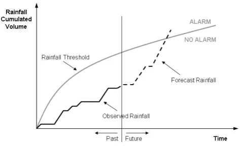
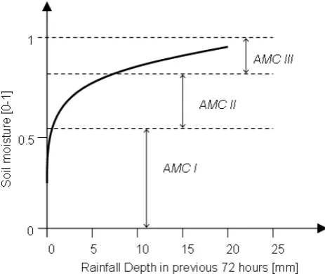
Fig. 1. Example of a rainfall threshold and its use.

1.2 The rainfall threshold approach

The use of rainfall thresholds is common in the context of landslides and debris flow hazard forecasting (Neary et al., 1986; Annunziati et al., 1996; Crosta and Frattini, 2000). Rainfall intensity increases surface landslide hazard (Crosta and Frattini, 2003) while soil moisture content affects slope stability (Iverson, 2000; Hennrich, 2000; Crosta et Frattini, 2001).

In the context of flood forecasting/warning, rainfall thresh-olds have been generally used by meteorological organiza-tions or by the Civil Protection Agencies to issue alerts. For instance, in Italy an alert is issued by the Civil Protection Agency if a storm event of more than 50 mm is forecast for the next 24 h over an area ranging from 2 to 50 km2. Unfortu-nately, this type of rainfall threshold, which does not account for the actual soil saturation conditions at the onset of a storm event, tends to heavily increase the number of false alarms.

In order to analyze flood warning rainfall thresholds in more detail, following the definition of thresholds used for landslides hazard forecast, let us define them as “the cumu-lated volume of rainfall during a storm event which can gen-erate a critical water stage (or discharge) at a specific river section”. Figure 1 shows an example of rainfall thresholds i.e. accumulated volume of rain versus time of rainfall accu-mulation. In order to establish the landslides warning thresh-olds, De Vita and Reichenbach (1998) use a number of statis-tics (such as the mean), to be derived from long historical records, of the amount of precipitation that happened imme-diately before the event.

Mancini et al. (2002), as an alternative to the use of his-torical records in the case of floods, proposed an approach based on synthetic hyetographs with different shapes and du-rations for the estimation of flood warning rainfall thresh-olds. The threshold values are estimated by trial and error with an event based rainfall-runoff model, as the value of rainfall producing a critical discharge or critical water stage. Although the Mancini et al. (2002) approach overcomes the limitations of the statistical analysis based exclusively on

historical records, rarely sufficiently long to produce statis-tically meaningful results, it presents some drawbacks due to the use of an event based hydrological model. In particular, it requires assumptions both on the temporal evolution of the designed storms and on the antecedent moisture conditions of the catchment, which one would like to avoid.

A rainfall threshold approach has also been developed and used within the U.S. National Weather Service (NWS) flash flood watch/warning programme (Carpenter et al., 1999). Flash flood warnings and watches are issued by local NWS Weather Forecast Offices (WFOs), based on the comparison of flash flood guidance (FFG) values with rainfall amounts. FFG refers generally to the volume of rain of a given du-ration necessary to cause minor flooding on small streams. Guidance values are determined by regional River Forecast Centers (RFCs) and provided to local WFOs for flood fore-casting and the issuance of flash flood watches and warnings. The basis of FFG is the computation of threshold runoff val-ues, or the amount of effective rainfall of a given duration that is necessary to cause minor flooding. Effective rainfall is the residual rainfall after losses due to infiltration, detention, and evaporation have been subtracted from the actual rain-fall: it is the portion of rainfall that becomes surface runoff at the catchment scale. The determination of FFG value in an operational context requires the development of (i) estimates of threshold runoff volume for various rainfall durations, and (ii) a relationship between rainfall and runoff as a function of the soil moisture conditions to be estimated for instance via a soil moisture accounting model (Sweeney et a., 1992).

than larger ones (Wang et al., 1981). But at the same time, the assumption of uniform rainfall excess over the whole catch-ment implicitly introduces upper bounds on the size of the catchments where a Unit Hydrograph approach could be con-sidered reasonable. Furthermore, the assumption of uniform rainfall excess over the catchment also implicitly limits the size of the catchment for which a unit hydrograph approach is reasonable.

With reference to the second aspect of the FFG, namely the estimation of the relationship between rainfall and runoff as a function of the soil moisture conditions, in a recent paper Georgakakos (2005) derives a relationship between actual rainfall and runoff, which is taken equal to the effective rain-fall, both for the operational Sacramento soil moisture ac-counting (SAC) model and for a simpler general saturation-excess model.

The results of this work have significant implications in operational application of the methodology. The threshold runoff is a function of the watershed surface geomorphologic characteristics and channel geometry but it also depends on the duration of the effective rainfall. This dependence im-plies one more relationship that must be invoked to determine the appropriate value and duration of the threshold runoff for any given initial soil moisture conditions. In other words op-erationally it is necessary to determine not only the relation-ship between the runoff thresholds and the flash flood guid-ance in terms of volumes but also in terms of their respective duration.

The method presented in this paper overcomes all the limitations due to historical records length, and the restric-tive linearity assumptions required by the Unit Hydrograph approach as well as the ones required by the Mancini et al. (2002) approach, by generating a long series of synthetic precipitation, which is then coupled to a continuous time Explicit Soil Moisture Accounting (ESMA) rainfall-runoff model. The use of continuous simulation, which necessar-ily implies continuous hydrological models of the ESMA type, was also advocated by Bras et al. (1985); Beven (1987); Cameron et al. (1999), and seems the most appropriate way for determining the statistical dependence of the rainfall-runoff relation to the initial soil moisture conditions. The sta-tistical analysis of the long series of synthetic results allows in development of joint and conditional probability func-tions, which are then used within a Bayesian context to de-termine the appropriate rainfall thresholds.

As presently implemented, the approach does not take into account the uncertainty in the quantitative precipitation fore-casts (QPF) provided by the numerical weather prediction (NWP) models. However, since the uncertainty of QPF is still quite substantial, an extension of the present approach is under development to incorporate this uncertainty by means of a Bayesian technique. Nonetheless, this first step was felt essential to demonstrate the feasibility of the proposed tech-nique with respect to the simple unconditional rainfall thresh-olds, i.e. independent from the initial soil moisture

condi-tions, which today are the basis for issuing warnings in many countries.

2 Description of the proposed methodology

In order to simplify the description of the methodology, two phases are here distinguished: (1) the rainfall thresholds es-timation phase and (2) the operational utilization phase. The first phase includes all the procedures aimed at estimating the rainfall thresholds related to the risk of exceeding a criti-cal water stage (or discharge) value at a river section. These procedures are executed just once for each river section of interest as well as for each forecasting horizon. The second phase includes all the operations to be carried out each time a significant storm is foreseen, in order to compare the precip-itation volume forecast by a meteorological model with the critical threshold value already determined in phase 1. 2.1 The rainfall thresholds estimation

As presented in Sect. 1.2, rainfall thresholds are here defined as the cumulated volume of rainfall during a storm event which can generate a critical water stage (or discharge) at a specific river section. When the rainfall threshold value is exceeded, the likelihood that the critical river level (or discharge) will be reached is high and consequently it be-comes appropriate to issue a flood alert; alternatively, no flood alert is going to be issued when the threshold level is not reached. In other words the rainfall thresholds must in-corporate a “convenient” dependence between the cumulated rainfall volume during the storm duration and the possible consequences on the water level or discharge in a river sec-tion. The term “convenient” is here used according to the meaning of the decision theory under uncertainty conditions, namely the decision which corresponds to the minimum (or the maximum) expected value of a Bayesian cost utility func-tion.

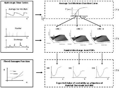
An-Fig. 2. Schematic representation of the proposed methodology. (1) Subdivision of the three synthetic time series according to the soil moisture conditions (AMC); (2) Estimation of the joint pdfs between rainfall volume and water stage or discharge; (3) Estimation of the “convenient” rainfall threshold based on the minimisation of the expected value of the associated utility function.

tecedent Moisture Condition (AMC) can be found in the lit-erature (Gray, 1982; Hawkins, 1985), which leads to the fol-lowing three classes of soil moisture AMC I (dry soil), AMC II (moderately saturated soil ) and AMC III (wet soil). Since each AMC class will condition the magnitude of the rainfall threshold, three threshold values have to be determined.

Given the loose link that can be found between rainfall totals and the corresponding water stages (or discharges) at a given river section, the estimation of the rainfall thresh-olds requires the derivation of the joint probability function of rainfall totals over the contributing area and water stages (or discharges) at the relevant river section. This derivation is based on the analysis of three continuous time series: (i) the precipitation averaged over the catchment area, (ii) the mean soil moisture value, (iii) the river stage (or the discharge) in the target river section. It is obvious that these time series must be sufficiently long (possibly more than 10 years) to ob-tain statistically meaningful results. In the more usual case when the historical time series are not long enough, the av-erage rainfall over the catchment is simulated by a stochastic rainfall generation model whose parameters are estimated on the basis of the observed historical time series. The rainfall stochastic model adopted in this work is the Neyman-Scott Rectangular Pulse NSRP model, widely documented in the

literature (Rodriguez-Iturbe et al., 1987a; Cowpertwait et al., 1996). With the above mentioned model, 10 000 years of hourly average rainfall over the catchment were generated and used as the forcing of a hydrologic model. The model used in this work is the lumped version of TOPKAPI (Todini and Ciarapica, 2002; Ciarapica and Todini, 2002; Liu and Todini, 2002). described in Appendix A with which the cor-responding 10 000 years of hourly discharges and soil mois-ture conditions have been generated.

At this point it is worthwhile noting that:

– The choice of the stochastic rainfall generation model and the rainfall-runoff model is absolutely arbitrary and does not affect the generality of the proposed method-ology.

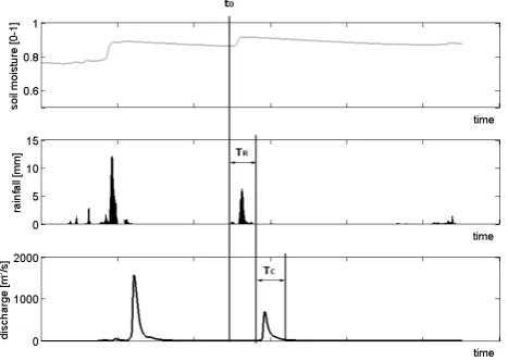
Fig. 3. The synthetic time series and the three time values used in the analysis:t0is the time of the storm arrival,T is the time interval

for the rainfall accumulation,TCis the time of concentration for the

catchment.

is generated by the meteorological models with a rather coarse resolution (generally larger than 7×7 km2). – The results obtained via simulation are not the threshold

values, but less stringent relations such as: (1) indicators incorporating the information on the mean soil moisture content, which are used to discriminate the appropriate AMC class and (2) the joint probability density func-tions between total rainfall over the catchment and the water stage (or discharge) at the river section of interest. Phase 1 of the proposed methodology for deriving the rain-fall thresholds follows the three steps illustrated in Fig. 2:

Step 1. Subdivision of the three time series obtained via simulation (generated average rainfall, simulated average soil moisture content, simulated water stage or discharge at the outlet) according to the defined soil moisture conditions (AMC) (Sect. 2.2);

Step 2. Estimation, for each of the identified AMC classes, of the joint probability density function of the rainfall cumu-lated over the forecasting horizon(s) of interest and the max-imum discharge in a related time interval (Sect. 2.3);

Step 3. Estimation of a rainfall alarm threshold, for each of the identified AMC classes (Sect. 2.4).

2.2 Step 1: Sorting the time series according to the AMC classes

In order to account for the different soil moisture initial con-ditions, it is necessary to divide the three synthetic records, namely the stochastically generated rainfall, the soil moisture conditions and the water levels (or discharges) obtained via simulation, in three subsets, each corresponding to a different AMC class.

This subdivision is performed on the basis of the AMC value relevant to the soil moisture condition preceding a

Fig. 4. A typical joint probability density function for rainfall volume and discharge with different (exponential and log-normal) marginal densities for a given soil moisture AMC class.

storm event. According to this value, the corresponding rain-fall and discharge time series will be grouped in the appro-priate AMC classes. This operation needs some further clar-ification, since the search for the rainfall totals and the cor-responding discharge (or water stage) must each be done in different time intervals in order to account for the catchment concentration time.

With reference to Fig. 3, three time values are defined:

t0 the storm starting time

T the rainfall accumulation time

TC the catchment concentration time

TC can be estimated from empirical relationships

based on the basin geomorphology or from time series analysis, when long records are available. As it emerged from the sensitivity analysis of the proposed methodology, in reality there is no need of great accuracy in the determination ofTC.

On the basis of the above defined time values, the rainfall volumeVT (or rainfall depth) accumulated fromt0tot0+T

and the maximum discharge valueQ(or the maximum water stage) occurring in the time interval fromt0tot0+T+TCare

retained and grouped in one of the classes according to the AMC value att0.

For a better description of the probability densities, al-though not essential, it was decided to construct the AMC classes so that they would each incorporate approximately the same number of joint observations. Therefore, the soil moisture contents corresponding to the 0.33 and 0.66 per-centiles can be used to discriminate among the three classes. Accordingly, based on the initial soil moisture condition at

t0, the different events are classified as AMC I (dry soil),

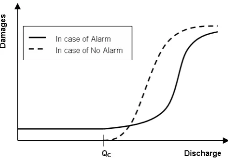
Fig. 5. Cost utility functions used to express the stakeholder per-ceptions.

Fig. 6. Expected value of the cost utility as a function of different rainfall threshold values. This analysis is repeated for each time rainfall accumulation time T and for each Antecedent Soil Moisture conditions class. For instance this graph is referred to AMC II and T=12 h.

2.3 Step 2: Fitting the joint probability density function Once the corresponding pairs of values (the rainfall total and the relevant maximum water stage or discharge) have been sorted into the three AMC classes, for each class one can use these values to determine the joint probability density func-tions (jpdf) between the rainfall total and the relevant maxi-mum discharge (or the water stage), to be used in step three. A jpdf will be estimated for each different forecasting hori-zonT, which will coincide with the rainfall accumulation time.

The problem of fitting a bi-variate density f (q, v|T )

in which marginal densities are vastly different (quasi log-normal for that of discharges and quasi exponential in terms

Fig. 7. Example of the rainfall thresholds derived for each AMC class as a function of rainfall accumulation time: when the soil is wet the threshold will obviously be lower.

Fig. 8. Box plot of the mean monthly soil moisture condition cal-culated using the TOPKAPI model for the Sieve catchment.

of rainfall totals) can be overcome either by using a “cop-ula” (Nelsen, 1999) or more interesting a Normal Quantile Transform (NQT) (Van der Waerten, 1952, 1953; Kelly and Krzysztofowicz, 1997). Figure 4 shows an example of the shape of one of the resulting bi-variate densities.

2.4 Step 3: Estimation of the most convenient rainfall threshold

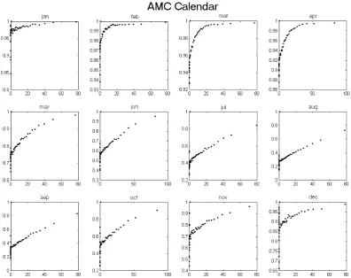
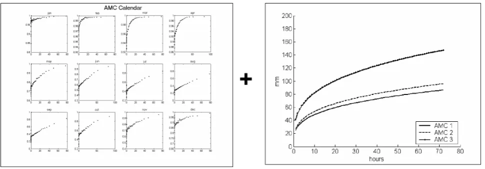
Fig. 9. The AMC calendar for the antecedent soil moisture condition estimation.

measurements rather than on their forecasts. Unfortunately, when dealing with smaller catchments, the flood forecasting horizon is mostly limited by the concentration time of the basin, which means that one has to forecast the discharges and the river stages as a function of the measured or casted precipitation. In this case, uncertainty affects the fore-casts and the problem of issuing an alert requires determin-ing the expected value of some utility or loss function. In the present work, following Bayesian decision theory (Ben-jamin and Cornell, 1970; Berger, 1986), the concept of “con-venience” is introduced as the minimum expected cost under uncertainty. The term “cost” does not refer to “actual costs” of flood damages that are probably impossible to be deter-mined, but rather a Bayesian utility function describing the damage perception of the stakeholder, which may even in-clude the non commensurable damages due to “missed alert”. Without loss of generality, in the present work the follow-ing cost function, graphically shown in Fig. 5, is expressed in terms of discharge:

U (q, v|VT, T )=

( a

1+be−c(q−Q∗) whenv≤VTand no alert is issued

C0+ a

0

1+b0_e−c0_(q−Q∗₎ whenv > VTand an alert is issued (1) withT the time of rainfall depth accumulation, v the

fore-casted volume and VT the rainfall threshold value, while

a, b, c anda0, b0, c0 are appropriate parameters. Due to the fact that the utility functions are only functional to the final objective of providing the decision makers with tools reflect-ing their risk perception, the shape of such functions, as well as the relevant parameter values, can be jointly assessed, by analysing the relevant effects on the decision process over past events.

U (q, v|VT, T )is the utility cost function, which ifv≤VT

expresses the perception of damages when no alert is issued (the dashed line in Fig. 5): no costs will occur if the discharge

qwill remain smaller than a critical valueQ∗, while damage costs will grow noticeably if the critical value is overtopped. On the contrary, ifv¿VT it expresses the perception of

dam-ages when the alert is issued (the solid line in Fig. 5) a cost which will be inevitably paid to issue the alert (evacuation costs, operational cost including personnel, machinery etc.), and damage costs growing less significantly when the criti-cal valueQ∗is overtopped and the flood occurs. As can be seen from Fig. 5, the utility function to be used will differ de-pending on the value of the cumulated rainfall forecastvand the rainfall thresholdVT. If the forecast precipitation value

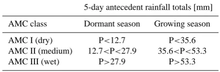
Table 1. AMC classes definition according to the SCS approach

5-day antecedent rainfall totals [mm] AMC class Dormant season Growing season AMC I (dry) P<12.7 P<35.6 AMC II (medium) 12.7<P<27.9 35.6<P<53.3 AMC III (wet) P>27.9 P>53.3

is greater than the threshold value, an alarm will be issued. The most “convenient” rainfall threshold value V_T∗ can thus be determined by search as the one that minimises the expected utility cost, namely:

V_T∗=Min

VT

hE{U (q, v|VT, T )}i

=Min

VT

Z +∞

0

Z +∞

0

U (q, v|VT, T ) f (q, v|T ) dq dv

(2) wheref (q, v|_{T )}is the joint probability distribution func-tion of the rainfall volume and the discharge peak value de-scribed in Sect. 2.3. One rainfall threshold value V_T∗ will be derived for each accumulation timeT. In Figure 6 one can see the typical shape of the expected value of the utility

E{U (q, v|VT, T )}for a given accumulation timeT.

Finally, Fig. 7 shows that all the values of the rainfall thresholds obtained for each AMC class, can be plotted as a function of the rainfall accumulation time. In the same Fig. 7, one can also appreciate the simplicity of the procedure used to decide whether or not to issue an alert. It is sufficient to progressively accumulate the forecast rainfall totals, starting from the measured rainfall volume and to compare the value to the appropriate AMC threshold value.

3 Operational use of the rainfall threshold approach

In order to operationally use the rainfall thresholds approach, whenever a storm event is forecast, one has to identify the AMC class to be used and the relevant rainfall threshold. This can be done without running a hydrological model in real time. For instance, in the cited work by Mancini et al. (2002), the AMC is estimated according to the Soil Con-servation Service definitions (SCS, 1986) reported in Table 1. However, the approach, although very simple, can lead to an incorrect estimation of the antecedent soil moisture, since it neglects the intra-annual long term dependency (season-ality) of the soil moisture conditions. As a matter of fact (see Table 1) the SCS AMC only incorporates the informa-tion relevant to the precipitainforma-tion of the previous 5 days, while from the example of Fig. 8, where the box plot of the mean monthly soil moisture condition is displayed, one can notice that the intra-annual variability of the soil moisture can be very high and the short-term influence of the precipitation

Table 2. Two-by-two contingency table for the assessment of a threshold based forecasting system

Forecasts

Observations Warning No Warning Total

W W0

Event,E h m e Non Event,E0 f c e0 Total w w0 n

alone is not sufficiently informative to correctly estimate the antecedent soil moisture conditions.

Therefore, an alternative methodology, which makes use of the long synthetic time series, already obtained for the thresholds derivation, is here proposed, to be applied only once in phase 1. As one can see from Fig. 9, it is possible to determine on a monthly basis, the simulated mean soil mois-ture as a function of the cumulated rainfall volume over the previousndays. More in detail, Fig. 9 shows for the Sieve catchment, on which the methodology was tested, the mean soil moisture of the month vs the precipitation volume cumu-lated over the previous 72 h. These results were obtained by using the 10 000 years synthetic rainfall and the correspond-ing simulated soil moisture series. The graphs in Fig. 9 will be referred to as the “AMC Calendar”. There is an evident dependency of the soil saturation condition on the antecedent precipitation and it is quite easy to estimate the appropriate AMC class by means of the AMC Calendar by comparing the cumulated rainfall value with the 0.33 and 0.66 quantiles determined as described in Sect. 2.2 (Fig. 10).

When a storm is forecast, using the rainfall thresholds to-gether with the AMC Calendar, it is possible to:

Determine the mean catchment soil moisture and the cor-rect AMC class, by entering into to the monthly graph with the cumulated rainfall volume recorded in the previousnh;

Choose the rainfall threshold corresponding to the identi-fied AMC class;

Add the forecast accumulated rainfall to the observed rain-fall volume;

Issue a flood alert if the identified threshold is overtopped.

4 A framework for testing the procedure

Fig. 10. The use of the monthly AMC Calendar to determine the appropriate AMC class.

A two-by-two contingency table can be constructed as illus-trated in Table 2. From a total number ofnobservations, one can distinguish the total number of event occurrences (e)and that of non-occurrences (e0); the total number of warnings is denoted asw, and that of no-warnings asw0. The following outcomes are possible: a hit, if an event occurred and a warn-ing was issued (withhthe total number of hits); a false alarm, if an event did not occur but a warning was issued (withf the total number of false alarms); a miss, if an event occurred but warning was not issued (withmthe total number of misses); a correct rejection, if an event did not occur and a warning was not issued (withcthe total number if correct rejections). The skill of a forecasting system can be represented on the basis of the hit rate and the false-alarm rate. Both ratios can be easily evaluated from the contingency table (Mason, 1982):

(

hit rate = h

h+m= h e

false-alarm rate = f f+c =

f e0

(3)

The hit and false-alarm rates (Eq. 3), indicate respectively the proportion of events for which a warning was provided cor-rectly, and the proportion of non events for which a warning was provided incorrectly. The hit rate is sometimes known as the probability of detection and provides an estimate of the probability that an event will be forewarned, while the false-alarm rate provides an estimate of the probability that a warning will be incorrectly issued (Eq. 4).

hit rate =p (W|E )

false-alarm rate =p WE0

(4)

For a system that has no skill, warnings and events are by definition independent occurrences, therefore, the

probabil-Fig. 11. The River Sieve catchment and the location of the different gauges.

ity of issuing an alert does not depend upon the occurrence or non occurrence of the event, namely:

p (W|E )=p WE 0

=p (W ) (5)

This equality occurs when warnings are issued at random. When the forecast system has some skill, the hit rate exceeds the alarm rate; a bad performance is indicated by false-alarm rate exceeding the hit rate. Because of the equality of the hit and false-alarm rates for all forecasts strategies with no skill, the difference between the two rate indexes can be considered an equitable skill score ss (Gandin and Murphy, 1992).

ss=p (W|E )−p WE0

(6)

5 The case study

Fig. 12. The three rainfall thresholds derived for the Sieve at For-nacina.

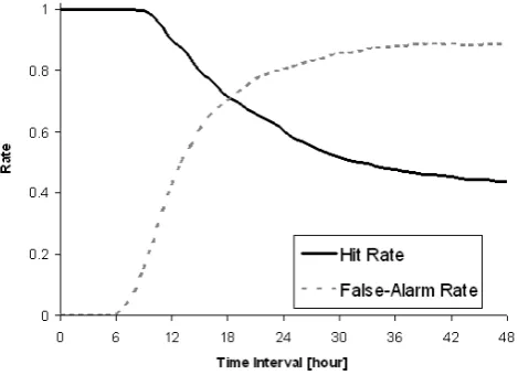
Fig. 13. Hit Rate and False-Alarm Rate as a function of flood fore-casting horizon for the case of the River Sieve at Fornacina.

obtained from surveys carried out in the last 10 years was also available. The conversion from water levels to river dis-charges at the Fornacina cross section is obtained by means of a rating curve, derived on the basis of flow velocity mea-sures and field surveys of the river cross section geometry, and provided by the Tuscany Regional Hydrological Service. According to the proposed methodology, a series of 10 000 years of hourly rainfall was generated by means of the Neyman-Scott Rectangular Pulse NSRP model (Rodriguez-Iturbe et al., 1987a; Cowpertwait et al., 1996). The generated rainfall was then used as input to the lumped TOPKAPI, a hydrological model described in Appendix A. The rainfall as well as the resulting discharges series were divided in three subsets (AMC1, AMC2, AMC3) according to the time se-ries of Antecedent Moisture Condition, also resulting from the hydrological simulation. “Convenient” rainfall threshold

Fig. 14. Skill score as a function of flood forecasting horizon for the case of the River Sieve at Fornacina.

values were then found by means of Eq. 2 for an increasing time horizonTranging from 0 to 72 h. Figure 12 shows the results obtained for the Sieve catchment at Fornacina.

The verification of the forecasting capabilities of the pro-posed methodology applied to the Sieve at Fornacina, based upon the validation framework described in Sect. 4, was per-formed by generating a 1000 year long time series of syn-thetic rainfall, different from the 10 000 year one used for setting up the methodological approach. The cases of Cor-rectly Issued Alarms (h), Missed Alarms (m), False Alarms (f ), Correctly Rejected Alarms (c)were computed for dif-ferent lead time horizons T. Based on the results, the hit rate and the false-alarm rate (Fig. 13) as well as the Skill Score (ss) (Fig. 14), were computed following their defini-tions given in Eq. 3 and Eq. 6 respectively as a function of accumulation timeT.

Fig. 15. The resulting two graphs on which the whole operational procedure of the proposed approach is based upon.

intensity events and long duration low intensity ones. Moreover, it must be borne in mind that these results do not incorporate the “rainfall forecasting uncertainty”. They were only derived, on the assumption of “perfect knowledge” of future rainfall, in order to validate the approach. In other words, the actually observed rainfall is here used as the “fore-casted rainfall”. In operational conditions, future rainfall is not known and only quantitative precipitation forecasts orig-inated either by nowcasting techniques or by Limited Area Atmospheric models may be available.

The introduction of a probabilistic rainfall forecast will inevitably imply the derivation of an additional probability densityf vvˆ

, expressing the probability of observing a given rainfall volume v conditional upon a forecasted vol-umevˆ, but it is envisaged that it will not completely modify the proposed procedure. Research work is currently under way to provide user oriented operational solutions and will be reported in a successive paper.

Nonetheless, it is worthwhile noting that the proposed methodology is very appealing for operational people. In fact, not only does it not require a flood forecasting model running in real time, but even a computer is not necessary in operational conditions: only the two graphs given in Fig. 15 are used in practice to evaluate the possibility of flooding. Therefore, the advantage of this method stems from its sim-plicity, thus providing a quick reference method to the stake-holders and the flood emergency managers interested at as-sessing, within a given lead time horizon, the possibility of flooding whenever a QPF is available.

6 Conclusions

This paper presented an original methodology aimed at is-suing flood warnings on the basis of rainfall thresholds. The rainfall threshold values relevant to a given river cross section take into account the upstream catchment initial soil moisture conditions as well as the stakeholders’ subjective perception

on the convenience of issuing an alert, through the minimiza-tion of expected costs, within the framework of a Bayesian approach. The advantage of the proposed methodology lies in its extremely simple operational procedure, based solely on two graphs, that makes it easy to be understood and ap-plied by non technical users, such as most flood emergency managers.

Nonetheless, not all the problems have been addressed for a successful operational use of the methodology. The pro-cedure presented in this paper, although it can be considered as a great improvement from the presently used approaches, must be viewed as a first step towards a sound operational approach. The limitation of the present stage is due to the implicit assumption of “perfect knowledge” of future rafall, in the sense that QPF is taken as a known quantity in-stead of an uncertain forecast. Although, this approach is currently used by most flood alert operational services, the role of the uncertainty in QPF has been presently brought to the attention of the community by meteorologists, through the use of ensemble forecasts and by meteorologists and hy-drologists within the frame of the recently launched Interna-tional Project HEPEX .

Ongoing research deals in fact with the problem of assess-ing uncertainty within the framework of the rainfall threshold approach.

The next step aims at incorporating the QPF uncertainty in the derivation of the rainfall thresholds, by taking the joint probability distribution function between rainfall and dis-charge (or water stage) derived via simulation as a distribu-tion condidistribu-tional on the knowledge of future rainfall. Given the probability density of future rainfall conditional on the QPF, it will then be possible to combine them in order to ob-tain the overall joint density from which one can integrate out the effect of the QPF uncertainty.

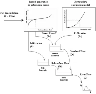
Fig. 16. The schematic representation of the lumped TOPKAPI hydrological model, according to Liu and Todini 2002l.

the effect of this uncertainty is much smaller on decisions than the one produced by the large QPF uncertainty.

Appendix A The rainfall-runoff model used: the lumped version of the TOPKAPI model

Two of the hydrologic time series used in the proposed methodology (namely the soil moisture content and the dis-charge at the river section of interest) were generated by means of a lumped rainfall-runoff model (the lumped version of TOPKAPI), which allows for a continuous simulation at an hourly time step.

The TOPKAPI approach is a comprehensive distributed-lumped approach widely documented in the literature (To-dini and Ciarapica, 2002; Ciarapica and To(To-dini, 2002; Liu and Todini, 2002). It was also shown (Liu and Todini, 2002), that the lumped TOPKAPI model schematized in Fig. 16, can be directly derived, without the need for a new calibra-tion, from the distributed physically meaningful version. In the lumped version, a catchment is regarded as a dynamic system composed of three reservoirs: the soil reservoir, the surface reservoir and the channel reservoir. The precipita-tion on the catchment is partiprecipita-tioned into direct runoff and

infiltration using a Beta-distribution curve, which reflects the non-linear relationship between the soil water storage and the saturated contributing area in the basin. The infiltration and direct runoff are then routed through the soil reservoir and surface reservoir, respectively. Outflows from the two reser-voirs, namely interflow and overland flow, are then taken as inputs to the channel reservoir to form the channel flow.

As previously mentioned, it can be proven that the lumped version of the TOPKAPI model can be derived directly from the results of the distributed version and does not require ad-ditional calibration. In order to obtain the lumped version of the TOPKAPI, the point kinematic wave equation is firstly integrated over the single grid cell of the DEM (Digital Ele-vation Model) and successively the resulting non-linear stor-age equation is integrated over all the cells describing the basin. In the case of the soil model the following relation is obtained:

∂VST

∂t =RA−



    

αs+1

αsX2

1

N−1 P

1=1 N−1

Q

m=`

f m

!

+1



     αs

XC¯STV as

with

1 ¯

CST =                N X

i=1                      1+ j−1

P j−1

Q

m=`

fm !

PN−1

` =1

N−1 Y

m=`

fm ! =1      

αs+1

αs −      

j−1 P

`=1 j−1

Q

m=` !

N=1 P

`=1 N−1

Q

m=`

fm ! =1      

αs+1

αs                , C 1 αs si                αs (A2)

whereiis the index of a generic cell;jis the of cells drained by theit hcell; N is the total number of cells in the upstream contributing area,VsT is the water storage in the catchment,

Ris the infiltration rate;Ais the catchment area; fm

repre-sents the fraction of the total outflow from themt hcell which flows towards the downstream cell, andαs is a soil model

parameter assumed constant in the catchment,bsis a lumped

soil reservoir parameter which incorporates in an aggregate way the topography and physical properties of the soil.

Equation A1 corresponds to a non-linear reservoir model and represents the lumped dynamics of the water stored in the soil. The same type of equation can be written for overland flow and for the drainage network, thus transforming the dis-tributed TOPKAPI model into a lumped model characterized by three “structurally similar” non-linear reservoirs, namely “soil reservoir”, “surface reservoir” and “channel reservoir”. Due to the spatial variability of the different cells in terms of water storage and flow dynamics, the infiltration rate in Eq. A1 must be preliminarily evaluated by separating precip-itation into direct runoff and infiltration into the soil. In order to obtain this separation, a relationship linking the extent of saturated areas and the volume stored in the catchment has to be introduced, similarly to what is done in the Xinanjiang model (Zhao, 1977), in the Probability Distributed Soil Ca-pacity model (Moore and Clarke, 1981) and in the ARNO model (Todini, 1996).

Given the availability of a distributed TOPKAPI version, this relationship can be obtained by means of simulation. At each step in time the number of saturated cells is put in re-lation to the total volume of water stored in the soil over the entire catchment. Indicating withV sTthe total water

stor-age in the soil, withV ss the soil water storage at saturation and withAsthe total saturated area, the relationship between

the extent of saturated areas and the volume stored in the catchment can be approximated by a Beta-distribution func-tion curve expressed by Eq. A3:

As A = VS_T VSS Z 0

0 (r+s) 0 (r) 0 (s)ϕ

r−1_(1−ϕ)s−1_{dϕ (A3)}

with0 (x)the Gamma function defined as:

0 (x)=

+∞ Z

0

ζx−1e−ζdζ , x>0 (A4)

As it was found in the analysis of the distributed TOPKAPI results, an exfiltration phenomenon exists. For instance when rainfall stops and the relevant overland flow has receded, sur-face runoff can still be larger that the possible maximum in-terflow due to a return flow caused by exfiltration. This return flow is estimated using a limiting parabolic curve (Fig. 16) representing the relationship between the return flow and the fraction of saturation in the catchment, which parameters are estimated on the basis of the distributed TOPKAPI model simulation results. This parabolic curve can be expressed as equation:

Qreturn=α1 _{V s}¯

T

V ss

2

+a2 ¯

V sT

V ss +α3 (A5)

whereQreturnis the calculated return flow discharge during

a time intervalt2−t1,V s¯ T=0.5CV sT1+V sT2is the averaged

soil water storage,a1, a2anda3are the parameters.

Accord-ingly, the infiltration rate into the soil within the time interval

1tcan be computed by using equation:

R= 1

A

_V

St₂ −VSt₁

t2−t1

−Qret

(A6)

The quantitiesRandRdare then input into the soil reservoir

and the surface reservoir, respectively. The interflow and the overland flow can be obtained by means of water balance method, and are then together drained into the channel reser-voir to generate the total outflow at the basin outlet (Fig. 16). For a more detailed description of the model refer to Liu and Todini, 2002.

Acknowledgements. The work described in this publication was supported by the European Community’s Sixth Framework Pro-gramme through the grant to the budget of the Integrated Project FLOODsite, Contract GOCE-CT-2004-505420. This paper reflects the authors’ views and not those of the European Community. Nei-ther the European Community nor any member of the FLOODsite Consortium is liable for any use of the information in this paper. Edited by: G. Pegram

References

Annunziati A., Focardi A., Focardi P., Martello S., and Vannocci P.: Analysis of the rainfall thresholds that induced debris flows in the area of Apuan Alps – Tuscany, Italy, Plinius Conference ’99: Mediterranean Storms, Ed. Bios., 485–493, 1999.

Benjamin, J. R. and Cornell C. A.: Probability, Statistics, and Deci-sion For Civil Engineers, McGraw-Hill, New York, 1970. Berger, J. O.: Statistical Decision Theory and Bayesian Analysis,

Beven, K.: Towards the use of catchment geomorphology in flood frequency predictions, Earth Surf. Processes Landforms, 12, 6– 82, 1987.

Bras, R. L., Gaboury D. R, Grossman D. S and Vicen G. J.: Spa-tially varying rainfall and flood risk analysis, J. Hydraul. Eng., 111, 754–773, 1985.

Cameron, D. S., K. J. Beven, J. Tawn, S. Blazkova, and P. Naden: Flood frequency estimation by continuous simulation for a gauged upland catchment (with uncertainty), J. Hydrol., 219, 169–187, 1999.

Carpenter, T. M., Sperfslage J. A., Georgakakos K. P., Sweeney T., and Fread D. L.: National threshold runoff estimation utilizing GIS in support of operational flash flood warning systems, J. Hy-drol., 224, 21–44, 1999.

Ciarapica L. and Todini E.: TOPKAPI: a model for the represen-tation of the rainfall-runoff process at different scales, Hydrol. Processes, 16(2), 207–229, 2002.

Cowpertwait P. S. P.: Further developments of the Neyman-Scott clustered point processes for modelling rainfall, Water Resour. Res., 27(7), 1431–1438, 1991.

Cowpertwait P. S. P., O’Connell P. E., Metcalfe A. V., and Mawds-ley J. A.: Stochastic point process modelling of rainfall, I. Single site fitting and validation, J. Hydrol., 175, 17–46, 1996. Crosta, G. B. and Frattini P.: Rainfall thresholds for soil slip and

debris flow triggering, Proceedings of the EGS 2nd Plinius Con-ference on Mediterranean Storms, Ed. Bios, 2000.

Crosta, G. B. and Frattini P.: Coupling empirical and physically based rainfall thresholds for shallow landslides forecasting, Pro-ceedings of the EGS 3rd Plinius Conference on Mediterranean Storms, Ed. Bios, 2001.

Crosta, G. B. and Frattini P.: Distributed modelling of shallow land-slides triggered by intense rainfall, Nat. Hazards Earth Syst. Sci., 3, 81–93, 2003.

EFFS: edited by: Gouweleeuw, B., Reggiani P., and de Roo, A., A European Flood Forecasting System, Full Report (Contract no. EVG1-CT-1999-00011, http://effs.wldelft.nl., 2004.

De Vita, P. and Reichenbach, P.: Rainfall triggered landslides: a reference list, Environ. Geol., 35(2/3), 219–233, 1998.

Gandin, L. S. and Murphy, A. H.: Equitable skill scores for cate-gorical forecasts, Mon. Wea. Rev., 120, 361–370, 1992. Georgakakos K. P.: Analytical results for operational flash flood

guidance, J. Hydrol., in press, 317, 81–103, 2006.

Gray, D. D., Katz, P. G., deMonsabert, S. M., and Cogo, N. P.: Antecedent moisture condition probabilities, J. Irrig. and Drain. Engrg. Div., ASCE, 108(2), 107–114, 1982.

Hawkins, R. H., Hjelmfelt, A. T., and Zevenberger, A. W.: Runoff probability, storm depth, and curve numbers, J. Irrig. and Drain. Engrg., ASCE, 111(4), 330–340, 1985.

Hennrich, K.: Modelling Critical Water Contents for Slope Stabil-ity and Associated Rainfall Thresholds using Computer Simu-lations, in: Landslides in Research, Theory and Practice edited by: Bromhead, E., Dixon, N., and Ibsen, M.-L.: Proceedings of the 8th International Symposium on Landslides, Cardiff/UK, Thomas Telford Ltd, 2000.

Iverson, R.M.: Landslide triggering by rain infiltration, Water Re-sour. Res., 36(7), 1897–1910, 2000.

Joe H.: Parametric families of multivariate distributions with given margins, J. Multivar. Anal., 46, 262–282, 1993.

Joe, H., Multivariate Models and Dependence Concepts, Chapman

& Hall, London, 1997

Kelly, K. S. and Krzysztofowicz, R.: A bivariate meta-Gaussian density for use in Hydrology, Stochastic Hydrology and Hy-draulics, 11, 17–31, 1997.

Lamb R. and Kay A. L.: Confidence intervals for a spa-tially generalized, continuous simulation flood frequency model for Great Britain, Water Resour. Res., 40, W07501, doi:10.1029/2003WR002428, 2004.

Liu Z. and Todini E.: Towards a comprehensive physically-based rainfall-runoff model, Hydrol. Earth Syst. Sci., 6, 859–881, 2002. Mancini M., Mazzetti P., Nativi S., Rabuffetti D., Ravazzani G., Amadio P., and Rosso R.: Definizione di soglie pluviometriche di piena per la realizzazione di un sistema di allertamento in tempo reale per il bacino dell’Arno a monte di Firenze, Proc. XXVII Convegno di idraulica e Costruzione Idrauliche, Volume, 2, 497– 505, Italy, 2002.

Mason, S. J.: A model for assessment of weather forecasts, Aust. Meteor. Mag., 30, 291–303, 1982.

Mason, S. J. and Graham, N. E.: Conditional Probabilities, Relative Operating Characteristics and Relative Operating Levels, Weat. Forecast., 14, 713–725, 1999.

Moore R. J. and Clarke R. T.: A distribution function approach to rainfall runoff modelling, Water Resour. Res., 17(5), 1367–1382, 1981.

Neary, D. G. and Swift L. W.: Rainfall thresholds for triggering a debris flow avalanching event in the southern Appalachian Mountains, Rew. Eng. Geol., 7, 81–95, 1987.

Nelsen, R. B.: An Introduction to Copulas, Springer-Verlag, New York, 1999.

Reed S., Johnson D., and Sweeney T.: Application and national Ge-ographic Information System database to support two-year flood and threshold runoff estimates, J. Hydrol. Eng., 7, 3, 1 May , 209–219, 2002.

Rodriguez-Iturbe I., Cox D. R., and Isham V.: Some models for rainfall based on stochastic point processes, Proc. R. Soc. Lon-don, Ser. A, 410, 269–288, 1987a.

Rodriguez-Iturbe I., Febres De Power B., and Valdes J. B.: Rect-angular Pulses point processes models for rainfall: analysis of empirical data, J. Geophys. Res., 92(D8), 9645–9656, 1987b. SCS – Soil Conservation Service: National Engineering Handbook,

sect. 4, Hydrology, Rev. Ed., U.S.D.A., Washington D.C., USA, 1986.

Sweeney, T. L.: Modernized areal flash flood guidance. NOAA Technical Report NWS HYDRO 44, Hydrologic Research Lab-oratory, National Weather Service, NOAA, Silver Spring, MD, October, 21 pp. and an appendix, 1992.

Todini E.: The ARNO rainfall-runoff model, J. Hydrol. ,175, 339– 382, 1996.

Todini E. and Ciarapica L.: The TOPKAPI model. In Mathematical Models of Large Watershed Hydrology edited by: Singh, V. P., Frevert, D. K., and Meyer, S. P., Water Resources Publications, Littleton, Colorado, Chapter 12, 471–506, 2002.

Van der Waerden, B. L.: Order tests for two-sample problem and their power, Indagationes Mathematicae, 14, 253–458, 1952. Wang, C. T., Gupta, V. K., and Waymire, E.: A geomorphologic

synthesis of nonlinearity in surface runoff, Water Resour. Res., 17(3), 545–554, 1981.