DECIDE, DETECT AND CLASSIFY BENIGN AND MALIGNANT IN
MAMMOGRAMS USING CV-PARTITIONING METHOD
BV. Kavetha and J. Venu Gopala Krishnan
Department of Electronics and Communication Engineering, Jeppiaar Engineering College, Chennai, India E-Mail: [email protected]
ABSTRACT
In recent years, the stage determining and classifying the mammogram as Benign or Malignant is somewhat complicated process in the medical research. In the earlier papers many classification techniques, CAD designs and feature extraction methods are used constantly for mammogram classification, and has its own advantages and limitations. To overcome the limitations, in this paper a novel approach is introduced for accurate classification of Benign and Malignant mammogram. This novel approach functions in three stages, where preprocess the image, decide the image in complete normal or Benign/Malignant and Determine whether the mammogram is Benign or Malignant by comparing the shape, color, texture and size of the extracted abnormal part of the mammogram Images. The experiment results give more than 99.3% of accuracy in classification by a MATLAB Programming method. The performance evaluation of the image is compared with the cv-partition method and feature extraction method.
Keywords: mammogram, benign, malignant, mammogram classification, normal, abnormal.
INTRODUCTION
A mammogram is an x-ray exam of the breast that’s used to detect and evaluate breast changes. X-rays were first used to examine breast tissue nearly a century ago, by the German surgeon, Albert Salomon. But modern mammography has only existed since the late 1960s, when special x-ray machines were designed and used just for breast imaging. Since then, the technology has advanced a lot, and today’s mammogram is very different even from those of the 1980s and 1990s.Today, the x-ray machines used for mammograms produce lower energy x-rays. These x-rays do not go through tissue as easily as those used for routine chest x-rays or x-rays of the arms or legs, and this improves the image quality. Mammograms today expose the breast to much less radiation compared with those in the past [1].
In many Western and American countries, breast cancer is the most common cancer among women. American National Cancer Institute reported that the population of the estimated new breast cancer cases for the 2008 in USA is round about179600, while the estimation of deaths is more than 40,700 [2]. These statistics claim that breast cancer held the second position of appearance in diagnosed new cases following prostate cancer compared with other forms of cancer. Over the past decades, it has become alarming that breast cancer incidence rates are increasing steadily. However, the mortality rates for breast cancer have remained relatively constant due to more effective treatment and earlier diagnosis [3]. Also, the United States has the highest crude and age standardized breast cancer incidences in the world: roughly 178,480 new cases of invasive breast cancer and 62,030 new cases of in situ breast cancer, 85% of which are ductal carcinoma in situ (DCIS), were diagnosed among American women in 2007 [2].
Related works
Intensive research work has been undertaken in the development of automated image analysis methods to assist radiologists in the identification of abnormalities. The role computers play in mammogram analysis is threefold: detection, diagnosis and noise cancellation. Detection involves identifying cancerous tissues in a mammogram. Early detection of breast cancer by mammography depends on the production of excellent images and competent interpretation. Mammography alone cannot prove that a suspicious area is malignant or benign. To decide that, the tissue has to be removed for examination using breast biopsy techniques. A false positive detection may cause an unnecessary biopsy. Some of the more important pitfalls encountered two decades ago with low contrast and poor image quality in mammography are presented in [4]. Diagnosis using mammograms is aimed at classifying the detected cancerous regions as benign or malignant. A review of several studies demonstrating how CAD tools help in tumor diagnosis is presented in [5].
the output of four spatial filters. Each feature vector was then classified using a binary decision tree.
Proposed approach
A novel approach is introduced, and it will decide the image is normal or abnormal, and detect the abnormal portion, then determine the mammogram belongs to benign mammogram or Malignant Mammogram. These three steps are explained in detail in fourth coming chapters.
The proposed system is divided into four major parts as shown in Figure-1:
Enhancement by using Histogram Equalization
Features Extraction
Classification
The detail of these four steps is described below one by one.
Problem statement
In this paper we tackle and solve the problem of finding and classifying the Benign and Malignant. The solution for this problem is given by the proposed approach which preprocesses the image and segment the image. From the segmented part of the mammogram, the novel approach detect, whether the mammogram is normal or abnormal. If the mammogram is normal there is no further precedence for classification, else the mammogram is analyzed from the segmented portion of the image by the shape of the image, texture, color and edge, and decide as a Benign or Malignant. After the deciding the mammograms as Benign or Malignant determine how many Benign, how many Malignant is available in the MIAS database. The step wise Detect, Decide and Determine approach is depicted pictorially in the following Figure-1.
Figure-1. System Architecture.
The overall functionality of the proposed approach is divided mainly into three steps, where the first step is pre-processing; the second step is segmentation and extraction of the affected portion of the mammogram images, the third step is analyzing the extracted portion’s shape, texture, color, intensity of the pixels. Due to these values the mammogram is Benign or Malignant will be decided.
Pre-Processing
The mammogram is read from the file and preprocessed by removing the noise using speckle noise removal method. For more accurate output, the mammogram image is enhanced using EM algorithm; convert the mammogram into gray scale if it is in RGB
color. After making the mammogram image as quality image, the segmentation is applied for deciding.
Speckle noise removal
Speckle noise is a granular noise that inherently exists in and degrades the quality of the active radar and synthetic aperture radar images and medical images. Reducing noise from the medical images; a satellite image etc. is a challenge for the researchers in digital image processing. Several approaches are there for noise reduction [12]. Generally speckle noise is commonly found in synthetic aperture radar images, satellite images and medical images.
An inherent characteristic of MRI imaging is the presence of speckle noise. Speckle noise is a random and
Read Test Mammogram Speckle Noise Removal Image Enhancement
RGB to Gray [Binary] Image Segmentation /
Extraction
Extracted Image Analysis [ check for Shape, color, texture and edge ]
Decide “Benign or εalignant”
deterministic in an image. Speckle has negative impact on ultrasound imaging, Radical reduction in contrast resolution may be responsible for the poor effective resolution of ultrasound as compared to MRI. In case of medical literatures, speckle noise is also known as texture. Generalized model of the speckle [13] is represented as,
(1)
Where, g(n, m) is the observed image, u(n, m) is the multiplicative component and (n,m)is the additive component of the speckle noise. Here n and m denotes the axial and lateral indices of the image samples. For the ultrasound imaging, only multiplicative component of the noise is to be considered and additive component of the noise is to be ignored. Hence, equation (1, 2) can be modified as;
Therefore, (2)
In this paper the speckle noise can be removed by alternatively select any sub option of median filter, wavelet filter and TV filter etc., Depends on the image and the image data the noise removal filter can be selected. Before removing the noise the image size is increased and padded as block kind of sub-image, and filter applied, hence the noise gets cleared completely.
where med(I) denotes the median filter applied on the image I.
Image enhancement using EM algorithm
The maximum likelihood ratio is estimated approximately by EM method [14], which has more attention because, the nature of the algorithm reckoning viability in tomographic image rebuilding [15~16], sign discovery [17] and stricture approximation [18]. Even though the EM algorithm is equally reckon for enhancing the image encountered in scanning, rendering and reproduction process. There is no existing methods reviewed can include the hypothetically multifaceted environment of numerous image formation procedures into a simple probability density array as EM procedure does. In this paper, a firmness improvement method exploiting EM procedure is proposed. By energetically giving a prior probability delivery suited for a specific application environment currently considered, the proposed method provides a general framework for rendering good image quality at the designated firmness for a large class of image development procedure.
In the EM procedure, a assumed, unobservable “complete data set” is working to ease the procedure of maximizing the likelihood function of the measured data. The actual cunning consists of a sequence of irregular anticipation steps and expansion steps. This iterative process has the necessary possessions of maximizing the likelihood function defined on the unhurried data monotonically, and meeting to a worldwide maximum at a unique point. A graphic illustration of the solicitation of the EM algorithm to firmness enhancement faced in the perusing process is showed in Figure-2. A glowing light source pulled by a resulting apparatus from top to bottom produces light on the shallow of the scanned hardcopy. The concentration of the light reproduced is then noticed by an array of light sensors. However, the intensity recorded by any specific sensor is affected not only by the area restricted by scanner firmness, but also adjacent areas due to the dispersal of light.
The proposed method exploiting EM technique can be used to recompense the above effect, reinstate the innovative density, or increase firmness if desired.
Figure-2. Enhanced image using EM algorithm.
The enhanced image using EM algorithm is depicted in Figure-2. The brightness of the image is increased and the tumor portion and the normal portion in the breast image is very clear on the image. Figure-2 is a resultant image where the EM algorithm is developed in Matlab and produced.
RGB2GRAY
The output of combing 30% of RED, 60% of GREEN and 11% of BLUE from an RGB image will be the gray scale image. The subsequent image will be 2D image. The significance 0 signifies black and the significance 255 signifies white. The variety will be between black and white values. The gray scale image is received by the using the equation (3)
Since RGB image has more key and more tenets from 0 to 255 in all the three colors. But in the gray it is abridged. Using the above gray formulation we change the color image into gray scale image. If the image handling procedures are applied on a gray scale, the result will be an accurate one.
Modified iterative watershed segmentation
Image separation is the separation of an image into sections or groups, which agree to dissimilar objects or parts of images. Every pixel in an image is owed to one of a quantity of these groups. A good separation is typically one in which:
Pixels in the same group have similar grey scale of multivariate values and form an associated section.
Adjacent pixels which are in dissimilar groups have dissimilar values.
The IWS technique is motivating when you have to describe an area which has neither texture nor gray level unity. Furthermore, this region should have ambiguous outlines and it should be problematic to section even by using human eyes. It is need to provide inner and outer indicators by using mouse clacks. Additionally your model is detailed; more precise will be the final separation. For the cancers we work on, the minimum number of clacks was of three inside and five outside, but it should depend on your image type.
The modified watershed segmentation algorithm is created by deriving and modifying the functionalities of the watershed segmentation algorithm. This method uses the gray scale mathematical morphology and segment the entire image into regions. MWS segmentation algorithm is also classified as region-based segmentation approach. Basically the nature of this algorithm developed to finds the flooded are by water in geographical system. In relation to the geographical environment, watershed catchment basin, watershed ridge-line, topological surface are concepts we are going to utilize in this paper for image segmentation. Mainly the input image is converted into another image where the objects can be identified in terms of regions. Due to improve the segmentation accuracy, the input image is converted into gray scale image, since the gray scale, eliminates the hue and saturation information while retaining the luminance. Next, the gray image is converted into binary image to segregate the image data as 0’s and 1’s. This helps to smoothen the image using morphological operations. The results obtained from modified watershed segmentation algorithm is shown in Figure-3.
Figure-3. Iterative modified watershed segmentation.
Image extraction by binary operation
The separated percentage of the image by iterative watershed segmentation can be mined by the two fold procedure. The Morphological operation is otherwise known as binary operation, where the operation is applied on the binary converted image. The mathematical morphology in image processing is particularly suitable for analyzing shapes in images. We introduce some basic concepts from set theory that is needed as substance for object localization used in this paper.
Let If be a subset of □2 and δ = {Lmin,...,Lmax} be an ordered set of grey levels. A grey-level image f can then be defined as a function:
f: If⊂□2→δ = {δmin,...,δmax }.
Furthermore, let B be a subset of □2and s∈□ a scaling factor, sB is structuring element B of size s, f is the maker, and g is the mask. We can write the basic morphological operations [19] as follows:
a) Dilation: [ ^((sB) ) (f)](x)= ǔmaxǕ_(b∈sB) f(xb) -5(a)
b) Erosion: [ ^((sB) ) (f)](x)= ǔminǕ_(b∈sB) f(xb) -5(b)
c) Opening: γ^((sB)) (f)= ^((sB) ) [ ^((sB) ) (f) -5(c)] d) Closing: ∅^((sB) ) (f)= ^((sB) ) [ ^((sB) ) (f)] - 5(d) e) Reconstruction: R_g (f)= _g^((i) ) (f)with _g^((i)) (f)= _g^((i+1)) (f),where
_g^((n) ) (f)= _g^((n-1) ) (f)with _g^((1) ) (f)= ^((b)) (f)∧g.
The equations 5(a,b,c,d) are the binary operation on the binary image which do un grouping, detecting, extracting and reconstruction an image.
Determine Benign or Malignant
Figure-4. Morphologic spectrum of masses [12].
A figure is well-defined as an interplanetary inhabiting lesion seen in at least two different forecasts [20]. If a possible figure is seen in only a single forecast it should be called 'Asymmetry' or 'Asymmetric Density' until its 3D is long-established. Figures have dissimilar density like fat containing, low density, iso dense and high density, different margins like circumscribed, micro lobular, obscured, indistinct and spiculated and different shape like round, oval, lobular, irregular.
Fat comprising radiolucent and mixed-density bounded lesions are benign, whereas isodense to high-density grassroots may be of benign or malignant origin [21]. Benign grazes tend to be iso dense or of low density, with very well defined limitations and enclosed by a fatty corona, but this is surely not analytic of benignancy. Iso dense means a flesh having alike to that of additional or adjacent flesh. The halo symbol is an acceptable radiolucent line that environs bounded grassroots and is highly prognostic that the figure is benign. Bounded boundaries are abruptly defined with an unexpected change over among the graze and then ear by flesh [22]. Without extra transformers there is nonentity to suggest penetration. A figure with bounded boundary is shown in Figure-5(a). Lesions with micro lobular boundaries have wavy contours. Covered margins of the figure are erased because of the superimposition with adjacent flesh. This term issued when the physician is persuaded that the figure is abruptly well-defined but has hidden boundaries. The poor description of unclear boundaries raises concern that there may be penetration by the lesion and this is not likely due to over laid normal breast tissue. The lesions with gambled boundaries are categorized by lines burning from the margins of a mass shown in Figure-5(b). A lesion that is ill-defined or gambled and in which there is no clear history of trauma to suggest hematoma or fat necrosis suggests a malignant procedure [21].
Figure-5. Examples of (a) circumscribed mass and (b) speculated mass [11].
Outline of a mass can describe it as benign or malignant. Masses with uneven outline usually designate malignancy as it is depicted in Figure-2. Regularly designed masses such as round and oval very often indicate a benign change.
Classification of Benign and Malignant
Mass analysis and classification
A typical benign mass has a round, smooth and well circumscribed boundary. On the other hand, a malignant tumor usually has a spiculated, rough and blurry boundary. However, there exist atypical cases of macro lobulated or spiculated benign masses, as well as micro lobulated or well circumscribed malignant tumors [23]. The detection of masses requires the segmentation of all possible suspicious regions, which may then be subjected to a series of tests to eliminate false positives.
Masses can have a range of sizes. Cancerous lesions are stochastic biologic phenomena that manifest in images as having various structures occurring at different sizes and over ranges of spatial scales [24]. The boundaries of masses require a localized approach, although the sharpness and hence the scales of interpretation of the lesion boundaries, can vary considerably. Moreover, the speculations that is associated with many cancerous lesions occur with different widths, lengths and densities, which suggest that their characterization will require analysis over scales.
Classification by CV-partition method
Create a classifier of cancer cells basing on the feature extracted from images of the samples. The complete set of data and the features consists of ID number, and a code M-for malignant, B for benign. The
real valued features are computed for each cell nucleus from the data. The computed values are radius, texture, perimeter, area, smoothness, compactness, contour portion and number o12f points on contour portion. Also the symmetry and the fractal dimension of each image data.
The complete functionality of the mammogram classification is given as a step wise procedure for computing in language is:
Read data file and assign it in an array
Get the size of the matrix
Cv partition (size(matrix)) // for training data and test it
The function Cv partition is used for Data partitions for cross-validation; it is an object of the Cv partition class defines a random partition on a set of data of a specified size. Use this partition to define test and training sets for validating a statistical model using cross-validation.
Feature comparison method
The features extracted in this study divided into two categories, one is shape based features and the other is the gray level features. The features are the Energy, Entropy, mean and Homogeneity of the image and those values retrieved from the image is compared with the threshold value which is predefined for Benign and Malignant. If the calculated values matched with the threshold value means it is decided that the image is malignant else it is benign.
Figure-6. Deciding the mammogram is Benign or Malignant.
RESULTS AND DISCUSSIONS
The complete proposed approach shown in the system architecture diagram is implemented in MATLAB-2012a software, and the stage wise result is given below. The input image is a local mammogram or it is from MIAS data base, is a benchmark database, has more than 200 images. Those images are in the gray scale and 2D images.
Figure-7. Noise removed input image.
Figure-8. Cancer detected.
Once the image noise removed and enhanced, the segmetnation process is applied on the image. The segmentation process, in this paper the iterative modified water shed segmentation is applied, to get the iterative
segmentaion on the image using various gray thresh old picked out in verious region on the image iteratively from the outside region to the center of the image is shown in Figure-8.
Figure-9. Extracted portion of the watershed segmentation.
We have used openly accessible databases MIAS. The dataset is occupied after the Mammographic Institute Society Analysis (MIAS). Every mammogram is of size 1024 x 1024 pixels, and resolution of 200 micron. There are 322 mammograms of right and left breast of 161
patients in this dataset. 69 mammograms were diagnosed as being benign, 54 malignant and 207 normal. Enhancement has been done by histogram equalization. Results have been shown in Figure-2.
The segmented portion of the mammogram is extracted from the original image and analysed due to the chape and the size and the color values of the iamge. According to the color [intensity], size, texture and the shape the detected tumor portion is named as ‘Benign or εalignant’ depicted in Figure-10.
Performance evaluation
There are three methods used for classification and their performance is compared by counting the number of perfect classification and number incorrect
classification as Benign and Malignant in the MIAS data base. In the three classification method the feature based classification method, written in MATLAB code, which extract the features of the image and compare the values with a predefined value, says the image is affected by Benign or Malignant.
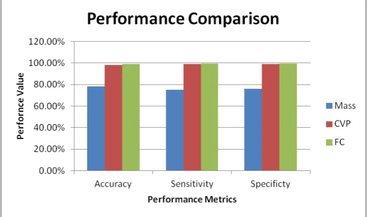
[image:8.595.117.479.398.612.2]We have tested the performance of the all the three methods [Mammogram Mass, CV-partition, Feature comparison] by calculating and analysis of accuracy, sensitivity and specificity for malignancy detection.
Table-1. Performance comparison of different classifiers.
Techniques Accuracy Sensitivity Specificity
Mammogram mass 78.45% 75.3% 76.2%
CV-Partition 98.24% 99% 99.2%
Feature comparison 99.3% 99.5% 99.6%
Performance of classifiers is calculated and analyzed by the following performance measures. Different classifier results are shown in Table-1. The
Feature comparison method gives more accuracy than the other techniques where it will classify by comparing the features with the threshold value.
Figure -11. Classified mammogram.
The accuracy of the Mammogram mass method is lesser than the cv-partition method and the cv-partition method gives lesser value than the feature comparison method. The feature comparison method’s accuracy is 99.3% according to the image dataset.
CONCLUSIONS
Proposed system is developed for diagnosing the breast cancer from mammogram images. This system performs this diagnosis in multiple phases. In first phase pre-processing on mammogram image is done to enhance
image quality. Then features extraction has been performed. Bayesian classifier has been used for classification. All experiments show that the proposed system gives exceptionally good results. In the future, we will perform to classify the malignancy of breast images by creating fractal model for fractal images.
REFERENCES
[2] Estimated New Cancer Cases and Deaths for 2008, http://seer. cancer.gov/cgi-bin/csr.
[3] M. J. M. Broeders and A. L. M. Verbeek. 1997. Breast cancer epidemiology and risk factors. Q-J-Nucl-Med. 41(3): 179-88.
[4] M. J. Homer. 1985. Breast imaging: pitfalls, controversies, and some practical thoughts. Radiologic Clinics of North America. 3: 459-472.
[5] Y. Jiang, R. M. Nishikawa, R. A. Schmidt, C. E. Metz, M. L. Giger and K. Doi. 1999. Improving breast cancer diagnosis with computer-aided diagnosis. Academic Radiology. 6: 22-33.
[6] H. P. Chan, K. Doi, C. J. Vyborny, K. L. Lam and R. A. Schmidt. 1988. \Computer-aided detection of microcalcications in mammograms: methodology and preliminary clinical study, Investigative Radiology. 23(9): 664-671.
[7] R. M. Nishikawa, M. L. Giger, K. Doi, C. J. Vyborny and R. A. Schmidt. 1995. \Computeraided detection of clustered microcalcications on digital mammograms, Medical and Biological Engineering and Computing. 33(2): 174-178.
[8] C. J. Vyborny and M. L. Giger. 1994. \Computer vision and artificial intelligence in mammography. American Journal of Roentgenology. 162(3): 699/708, March.
[9] W. P. Kegelmeyer, Jr. 1992. \Computer detection of stellate lesions in mammograms. Proceedings of the SPIE Conference on Biomedical Image Processing and Three Dimensional Microscopy. San Jose, California. pp. 446-454.
[10]D. Brzakovic, X. M. Luo, and P. Brzakovic. 1990. \An approach to automated detection of tumors in mammograms. IEEE Transactions on Medical Imaging. 9(3): 233-241.
[11]W. P. Kegelmeyer, Jr., J. M. Pruneda, P. D. Bourland, A. Hillis, M. W. Riggs and M. L. Nipper. 1994. \Computer-aided mammographic screening for spiculated lesions. Radiology. 191(2): 331-336.
[12]Milindkumar V. Sarode, Prashant R. Deshmukh. Reduction of Speckle Noise and Image Enhancement of Images Using Filtering Technique. International
Journal of Advancements in Technology http://ijict.org/ ISSN 0976-4860.
[13]K. Thangavel, R. Manavalan, Laurence Aroquiaraj. 2009. Removal of Speckle Noise from Ultrasound Medical Image based on Special Filters: Comarative study. ICGST-GVIP Journal. 9(3): 25-32.
[14]A. P. Dempster, N. M. Laird and D. B. Rubin. 1977. Maximum Likelihood from Incomplete Data via the EM Algorithm. JRSS. 39: 1-38.
[15]L. A. Shepp and T. Vardi. 1982. Maximum Likelihood Reconstruction for Emission Tomography. IEEE Trans. Med. Imaging. MI-1: 113-122.
[16]M. I. Miller, D. C. Snyder and T. R. Miller. 1985. Maximum Likelihood Reconstruction for Single-Photon Emission Computed Tomography. IEEE Trans. Nucl. Sci. NS-32: 769-778.
[17]C. N. Georghiades, D. L. Snyder. 1991. The Expectation-Maximization Algorithm for Symbol Unsynchronized Sequence Detection. IEEE Trans. Commun. 39(1): 54-61.
[18]M. Feder and E. Weinstein. 1988. Parameter Estimation of Superimposed Signals Using the EM Algorithm. IEEE Trans. Acoust., Speech, Signal Processing. 36(4): 477-489.
[19]Kittipol Wisaeng, Department of Computer Science. 2012. Automatic Optic Disc Detection from Low Contrast Retinal Images. Applied Mathematical Sciences. 6(103): 5127-5136.
[20]American College of Radiology (ACR). 2003. ACR Breast Imaging Reporting and Data System. Breast Imaging Atlas, 4th Edition, Reston, VA. USA.
[21]E.S. de Paredes. 2007. Atlas of Mammography. 3rd Edition, Lippincott Williams and Wilkins, Philadelphia, USA.
[22]H. Zonderland. BI-RADS - Introduction to the Breast Imaging Reporting and Data System. [Online] Available: www.radiologyassistant.nl
[24]A.C. Bovik. 2005. Handbook of Image and Video Processing. Elsevier Academic Press, Amsterdam, 2005