The Comparison between Random Forest and Support
Vector Machine Algorithm for Predicting
β
-Hairpin Motifs
in Proteins
*
Shaochun Jia, Xiuzhen Hu, Lixia Sun
Department of Physics, College of Sciences Inner Mongolia University of Technology, Huhhot, China Email: [email protected]
Received 2013
ABSTRACT
Based on the research of predicting β-hairpin motifs in proteins, we apply Random Forest and Support Vector Machine algorithm to predict β-hairpin motifs in ArchDB40 dataset. The motifs with the loop length of 2 to 8 amino acid resi-dues are extracted as research object and the fixed-length pattern of 12 amino acids are selected. When using the same characteristic parameters and the same test method, Random Forest algorithm is more effective than Support Vector Machine. In addition, because of Random Forest algorithm doesn’t produce overfitting phenomenon while the dimen-sion of characteristic parameters is higher, we use Random Forest based on higher dimendimen-sion characteristic parameters to predict β-hairpin motifs. The better prediction results are obtained; the overall accuracy and Matthew’s correlation coefficient of 5-fold cross-validation achieve 83.3% and 0.59, respectively.
Keywords: Random Forest Algorithm; Support Vector Machine Algorithm; β-Hairpin Motif; Increment of Diversity; Scoring Function; Predicted Secondary Structure Information
1. Introduction
β-hairpin is a super secondary structure motif. In the β-β motif, if two anti-parallel β-strands are connected by loop and there are one or more hydrogen bonds between two adjacent strands, then the structure is called as β-hairpin [1-3], otherwise it is considered as non-β-hairpin. Correct prediction of β-hairpin motifs is helpful to folding recog-nition, and it is vital for simplifying folding numbers of unknown structure [4-6]. Therefore prediction of β-hair- pin motifs has very important meaning.
In the past few years, some methods have been devel-oped for predicting β-hairpin motifs in different datasets and better prediction results were obtained. In 2002, Cruz
et al. [2] employed an artificial neural network (ANN) for predicting β-hairpins in 534 protein chains; an accu-racy of 47.7% was obtained. In 2004, Kuhn et al. [1] also used ANN for predicting hairpins in 2209 protein chains by identifying local hairpins and non-local diverging turns; an accuracy of 75.9% was achieved. In 2005, Ku-mar et al. [3] used a Support Vector Machine (SVM) and ANN technique to predict β-hairpins in 2880 no redun-
dant protein chains and obtained an accuracy of 79.2%. In 2008, our group’s Hu [7] et al. predicted β-hairpins in ArchDB40 dataset by using SVM, the overall accuracy and Matthew’s correlation coefficients are 79.9% and 0.59, respectively. In 2010, our group’s Hu et al. [8] at-tempted to use a quadratic discriminate (QD) method for predicting β-hairpins in ArchDB40 dataset, the overall accuracy and Matthew’s correlation coefficients are 81.6% and 0.55, respectively.
In this article, we attempt to use a combination clas-sifier algorithm, Random Forest and Support Vector Ma-chine to predict β-hairpin motifs in ArchDB40 dataset. By using of the composite vector with increment of di-versity, scoring function and predicted secondary struc-ture information as characteristic parameters. When us-ing Random Forest as prediction algorithm, the overall accuracy and Matthew’s correlation coefficient of 5-fold cross-validation achieve 82.0% and 0.55, respectively. However, when Support Vector Machine is used as pre-diction algorithm, they are only 79.4% and 0.49, respec-tively. Similarly, the results of Random Forest algorithm are also better than Support Vector Machine for the in-dependent test. Furthermore, we also use Random Forest based on higher dimension characteristic parameters to predict β-hairpin motifs. The prediction results are fur-ther improved.
*National Natural Science Foundation of China (30960090).
Natural Science Foundation of the Inner Mongolia of China (project No.2009MS0111).
2. Materials and Methods
1) Materials
Our algorithm is trained and tested on ArchDB40 da-taset. That is generated from ArchDB, in which the clas-sification of protein loops from no redundant proteins of known structures
(http://www.sbi.imim.es/cgi-bin/archdb/loops.pl). ArchDB was based on DSSP [9] database and provided by Oliva et al. [10,11]. ArchDB40 subset contains 3,088 no redundant proteins with resolution <3.0 Å, in which no two protein chains have a percentage identity >40% (ASTRAL SCOP 1.65). The ArchDB40 subset contains 9180 β-β motifs are divided into 6216 β-hairpin motifs and 2964 non-β-hairpin motifs. Here a total of 6028 β- hairpin motifs and 2643 non-β-hairpin motifs with the loop length of 2 to 8 amino acid residues are selected as research object.
2)Methods
a) Random Forest (RF) Algorithm.
Random Forest that had been originally proposed by Leo Breiman [12] in 2001 is an ensemble classifier, it contains many decision trees. For each tree in the forest, a training set is firstly generated by randomly choosing N
times with replacement from all N samples of the original dataset (bootstrap), and the rest are used as a testing set. When each node of single decision tree is splitting, the number of features used for splitting each node of deci-sion tree (m) is firstly specified. Then m out of M
features are randomly selected and the best split attribute on these m features is used to split the node, such that the impurity at each node of single decision tree is mini-mized and each tree in the forest fully grows without pruning. A Random Forest with k decision trees is formed by repeating k times as above procedure, and then the Random Forest is used to predict test data. The final classification results are decided by all the votes [13,14].
Random Forest has two most significant parameters, one is the number of features used for splitting each node of decision tree (m, m M where M is the total num-ber of features), another parameter is the numnum-ber of trees (k). In this work, and m is equal to M , k is equal to 500. Random Forest algorithm is implemented by using the package in R software [15] (http://www.r-project.org/). One obvious properties of the algorithm is that it doesn’t produce overfitting phenomenon when the characteristic parameters of higher dimension are used.
b)Support Vector Machine (SVM) Algorithm.
The Support Vector Machine (SVM) is a promising binary classification method developed by Vapnik [16]. As a supervise machine learning technology, the algo-rithm had been used for many kinds of pattern recogni-tion problems. In addirecogni-tion, because the algorithm of Support Vector Machine is a convex quadratic optimiza-tion problem, the local optimal soluoptimiza-tion is certainly the
global optimal one. But other algorithms (such as ANN) don’t have these features of SVM. In this paper, we use SVM to predict β-hairpin motifs. SVM has been widely used by transforming the input vector into a high-di- mension Hilbert space and seeking a separating hyper-plane in this space. The form of the decision function is:
( )
(
)
1
sgn
N
i i i
i
f x α∗y K x x b∗
=
= ⋅ +
∑
(1)In this paper, we select the radial basis kernel function (RBF) (K x x
(
i⋅)
=exp(−g xi−x2)). The optimal val-ues of parameters C and g are default. SVM has been compiled into the software packages; we use libsvm-2.89 SVM software packages(http://www.csie.ntu.edu.tw/~cjlin/libsvm). 3) The Selection of the Characteristic Parameters a) The Selection of the Fixed-length Pattern
According to Hu’s [7] ideas, β-hairpin motifs with the loop length of 2 to 8 amino acid residues in the dataset are extracted as research object and the fixed-length pat-tern of 12 amino acids are selected. Particular rules de-scribed as below:
i) The first amino acid (beginning) of loop locates the fifth position of the fixed-length pattern (5 - 12).
ii) End of loop locates the eighth position of the fixed-length pattern (8 - 12).
iii) The loop locates the center of fixed-length pattern. If the loop length is odd, the central coil is mapped and six residues (excluding the central coil) from the left- hand side and five residues from the right-hand side are taken. If not, the central two coils are mapped and five residues (excluding the central two coils) from both the sides were taken (Lr-12).
For above three rulers, if pattern length was <12, resi-dues flanking the peptide in the amino acid sequence were appended at both the ends.
b) Amino acids component of position (A)
We statistically analyze the amino acid compositions at 12 positions of the fixed-length pattern of β-hairpin and non-β-hairpin motifs. The results show that conser-vation of position is stronger in the fixed-length sequence fragments. So amino acids component of position is ex-tracted as sequence information. Because of the fixed- length pattern are generated using three rules, amino ac-ids component of position is described as a vector of 21 × 12 dimensions (21 denotes 20 amino acids and one ter-minal residue) for each ruler.
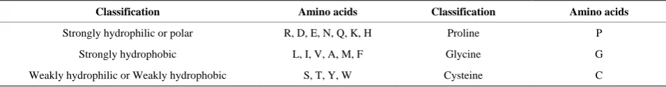
c)Hydropathy component of position (Q)
Table 1. Hydropathy characteristics for 20 amino acids.
Classification Amino acids Classification Amino acids
Strongly hydrophilic or polar R, D, E, N, Q, K, H Proline P
Strongly hydrophobic L, I, V, A, M, F Glycine G
Weakly hydrophilic or Weakly hydrophobic S, T, Y, W Cysteine C
minal residue) for each ruler, classification of hydropathy characteristics [17] for 20 amino acids are showed in Ta- ble 1.
d) Increment of Diversity(ID)
In the state space of s dimension, the diversity measure for diversity sources S: {m1, m2… ms} is defined as [18]:
( ) log ilog i i
D S =M M−
∑
m m (2)In the same state space, increment of diversity between the source of diversity X: {n1, n2,… ns} and Y: {m1, m2… ms} is defined as:
( , )
( ) log( ) ( ) log( )
log log log log
i i i i
i
i i i i
i i
ID X Y
M N M N m n m n
M M N N m m n n
= + + − + +
− − + +
∑
∑
∑
(3)
Here i, i
i i
N =
∑
n M =∑
m . Amino acids component of position is selected as the basic parameter, and then constructs 2 diversity sources for β-hairpin and non-β- hairpin motifs. Because of the fixed-length pattern are generated using three rules, arbitrary sequence segments can obtain 6 ID values (ID (A)) which be calculated by Equation (3). Similarly, hydropathy component of position is also selected as the basic parameter. Arbitrary sequence segments obtain 6 ID values (ID (Q)) which be calculat- ed by Equation (3).e) Scoring function(S)
The position weight scoring function is a simple but effective forecast algorithm. Here we only calculate the scores of β-hairpin and non-β-hairpin motifs as characte-ristic parameters, the score of segment can be defined as [19]:
(4)
(5)
(6)
(7)
Where j is amino acid j or terminal residue, Ni is the
number of amino acids and terminal residue at the posi-tion i, nij is the number of amino acid j or terminal
resi-due at the position i, wi, min and wi, max are the minimal
and maximal values of position weight at the position i, respectively. wij is the observed position weight at the
position i, Ci is the conservation index vector at position i.
Amino acids component of position is selected as the basic parameter. Because of the fixed-length pattern are generated using three rules, arbitrary sequence segments can obtain 6 S values (S12 (A)) which be calculated by Equation (4).
f) Predicted secondary structure information (SS) In the research of predicting β-hairpin motifs, litera-ture [2,3] had used predicted secondary struclitera-ture infor-mation as the characteristic parameters; better prediction results were obtained. In order to improve the prediction effect, we also extract predicted secondary structure in-formation. These are obtained by using the PHD [2] soft-ware, and are represented by a vector of 3 dimensions which are the frequency of predicted secondary structure (α-helix, β-sheet and coils).
3. Results and Discussion
1) Performance Measures
In order to evaluate the correct prediction rate and the reliability of a predictive method, we use the following standard measures. Accuracy of prediction (Acc); Mat-thew’s correlation coefficient (MCC); sensitivity of
β-hairpin (Qo H( )); sensitivity of non-β-hairpin prediction
(Qo NH( )); specificity of β-hairpin prediction (Qp H( ));
specificity of non-β-hairpin (Qp NH( )) [7]; calculating
formula as follow:
( ) 100%
( )
p r Acc
p r o u
+
= + + + ×
(8)
[( ) ( )]
( )( )( )( )
p r o u MCC
p u p o r u r o
× − × =
+ + + + (9)
( ) ( ) 100%
o H p Q p u = + ×
(10)
( ) ( ) 100%
o NH r
Q
r o
= + ×
(11)
( ) ( ) 100%
p H p Q p o = + ×
(12)
12 ,min 1 12 ,max ,min 1 ( ) ( )
i ij i i
i i i
i
C w w
S
C w w
= = − = −
∑
∑
0log( ij )
ij j p w P = 21 1
100 ( log log 21)
log 21
i ij ij
j
C P p
( ) ( ) 100%
p NH r
Q
r u
= + ×
(13)
Here p and r denote the number of correctly predicted
β-hairpin and non-β-hairpin, respectively; u denotes the number of the β-hairpin that are predicted as non-β-hair- pin, o denotes the number of the non-β-hairpin that are predicted as β-hairpin.
2) The Predictive Results Using of 5-fold Cross-vali- dation
By using of the composite vector with increment of diversity (ID(A) + ID(Q)), scoring function (S12(A)) and predicted secondary structure information (SS) as cha-racteristic parameters. When RF algorithm is applied to predict β-hairpins, for 5-fold cross-validation, Acc and
MCC are 82.0% and 0.55, respectively. However, when SVM is used as prediction algorithm, Acc and MCC are only 79.4% and 0.49, respectively. Besides, the Qo(H), Qo(NH), Qp(H), and Qp(NH) of RF algorithm are all higher
than SVM. The results show that RF algorithm is better than SVM. In addition, to compare our method with oth-ers, we also list previous prediction results in Table 2. It can be seen that our prediction overall accuracy of using RF algorithm is slightly higher than Hu’s [7,8] results. But the Matthew’s correlation coefficient is lower than Hu’s [7,8] results.
3) The Predictive Results Using of the independent test To further compare RF and SVM algorithm, we also use the independent test. The 1028 β-hairpins and 643 non-β-hairpins are selected as training set from 6028
β-hairpins and 2643 non-β-hairpins, the remaining 5000
β-hairpins and 2000 non-β-hairpins are independent test-ing set. By ustest-ing of the composite vector (ID (A) + ID(Q) + S12(A) + SS) as the characteristic parameters, when RF algorithm is applied to predict β-hairpin motifs. Acc
and MCC are 79.9% and 0.50, respectively. However,
when SVM algorithm is used as prediction algorithm,
Acc and MCC are only 77.0% and 0.43, respectively. Predictive results are showed in Table 3. It can be seen that RF algorithm is still better than SVM. Furthermore, it should be noticed that using the small sample to test the large one in here.
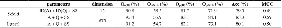
4) The Predictive Results Using of higher dimension characteristic parameters
Considering the obvious properties of RF algorithm, we directly use the composite vector with amino acids component of position (A), hydropaths component of po-sition (Q), and predicted secondary structure information (SS) as characteristic parameters (675 dimensions). Acc
[image:4.595.54.542.539.599.2]and MCC of 5-fold cross-validation achieve 83.3% and 0.59, respectively. It needs to be pointed out that, amino acids component of position and hydropaths component of position are only based on the first two cutting rules (5 - 12, 8 - 12) in here. In contrast, we also use of the com-posite vector (ID(A) + ID(Q) + SS) as the characteristic parameters. Acc and MCC of 5-fold cross-validation are 79.5% and 0.49, respectively. The predictive results are decreased. Then we use RF algorithm based on the com-posite vector (A + Q + SS) to predict β-hairpin motifs. For the independent test (I (test)), Acc and MCC are 80.1% and 0.50, respectively. Predictive results are showed in
Table 4. The results indicate that 5-fold cross-validation and the independent test are similar when RF algorithm is used to predict β-hairpin motifs.
4. Conclusion
In this paper, the predictive results of using RF algorithm based on the composite vector (A + Q + SS) are better than previous. From above results we can seen: 1) RF algorithm is better than SVM when the same characteris-tic parameters and the same test method are used; 2) Due
Table 2. Predictive results using of 5-fold cross validation for β-hairpinsand non β-hairpins in ArchDB40 dataset. Method (parameters) Qo(H) (%) Qo(NH) (%) Qp(H) (%) Qp(NH) (%) Acc (%) MCC
RF(ID(A), ID(Q), S12 (A), SS) 92.0 59.2 83.7 76.4 82.0 0.55
SVM(ID(A), ID(Q), S12 (A), SS) 89.1 57.3 82.6 69.7 79.4 0.49
SVM(S, ID) [7] 80.3 79.3 86.1 71.5 79.9 0.59
[image:4.595.59.538.625.660.2]QD(S12(a), ID(aa), ID(qq), ID(Af)) [8] 89.1 64.7 85.2 72.2 81.6 0.55
Table 3. Predictive results using of the independent test for β-hairpins and non β-hairpins in ArchDB40 dataset. Method(parameters) Qo(H) (%) Qo(NH) (%) Qp(H) (%) Qp(NH) (%) Acc (%) MCC
RF(ID(A), ID(Q), S12(A), SS) 91.2 54.1 81.9 72.9 79.9 0.50
[image:4.595.60.540.688.736.2]SVM(ID(A), ID(Q), S12(A), SS) 87.9 52.1 80.7 65.5 77.0 0.43
Table 4. Predictive results using Random Forest algorithm for β-hairpins and non β-hairpins in ArchDB40datase. parameters dimension Qo(H) (%) Qo(NH) (%) Qp(H) (%) Qp(NH) (%) Acc (%) MCC
5-fold ID(A) + ID(Q) + SS 15 90.8 53.5 81.7 71.9 79.5 0.49
A + Q + SS
675 95.4 55.9 83.1 84.1 83.3 0.59
to RF algorithm doesn’t produce overfitting when the dimension of the characteristic parameters is higher, bet-ter results are still obtained. But the phenomenon will appear in this case for the SVM; 3) Previous independent test is usually that using the large sample to test the small one. However, we still obtain better predictive results by using the small sample to test the large one when RF algorithm is used. This implies that RF algorithm is steady and effective.
REFERENCES
[1] M. Kuhn, J. Meiler and D. Baker, “Strand-Loop-Strand Motifs: Prediction of Hairpins and Diverging Turns in Proteins,” Proteins: Structure, Function, and Bioinforma- tics, Vol. 54, 2004, pp. 282-288.
[2] X. Cruz, E. G. Hutchinson, A. Shepherd and J. M. Thorn- ton, “Toward Predicting Protein Topology: An Approach to Identifying β Hairpins,” Proceedings of the National Academy of Sciences of the USA, Vol. 99, 2002, pp.
11157-11162.
[3] M. Kumar, M. Bhasin, N. K. Natt and G. P. S. Raghava, “BhairPred: Prediction of β-Hairpins in a Protein from Multiple Alignment Information Using ANN and SVM Techniques,” Nucleic Acids Research, Vol. 33, 2005, pp.
154-159.
[4] T. F. Jenny, D. L. Gerloff, M. A. Cohen and S. A. Benner, “Predicted Secondary and Super Secondary Structure for the Serine-Threonine-Specific Protein Phosphatase Fam-ily,” Proteins: Structure, Function, and Bioinformatics, Vol. 21, 1995, pp. l-10.
[5] A. Godzik, J. Skolnick and A. Kolinski, “Simulations of the Folding Pathway of Triose Phosphate Isomerase-Type Alpha/Beta Barrel Proteins,” Proceedings of the National Academy of Sciences of the USA, Vol. 89, 1992, pp.
2629-
[6] R. T. Wintjens, M. J. Rooman and S. J. Wodak, “Auto-matic Classification and Analysis of Alpha Alpha-Turn Motifs in Proteins,” Journal of Molecular Biology, Vol. 255, 1996, pp. 235-253.
[7] X. Z. Hu and Q. Z. Li, “Prediction of the β-Hairpins in Proteins Using Support Vector Machine,” Protein Jour- nal, Vol. 27, 2008, pp. 115-122.
[8] X. Z. Hu, Q. Z. Li and C. L. Wang, “Recognition of β- Hairpin Motifs in Proteins by Using the Composite Vec-
tor,” Amino Acids, Vol. 38, 2010, pp. 915-921.
[9] W. Kabsch and C. Sander, “Dictionary of Protein Secon- dary Structure: Pattern Recognition of Hydrogen-Bonded and Geometrical Features,” Biopolymers, Vol. 22, 1983,
pp. 2577-2637
[10] B. Oliva, P. A. Bates, E. Querol, F. X. Aviles and M. J. E. Sternberg, “An Automated Classification of the Structure of Protein Loops,” Journal of Molecular Biology, Vol. 266, 1997, pp. 814-830.
[11] J. Espadaler, N. F. Fuentes, A. Hermoso, E. Querol, F. X. Aviles, M. J. E. Sternberg and B. Oliva, “ArchDB: Auto- mated Protein Loop Classification as a Tool for Structural Genomics,” Nucleic Acids Research, Vol. 32, 2004, pp.
185-
[12] L. Breiman, “Random Forests,” Machine Learning, Vol. 45, 2001, pp. 5-32.
[13] F. S. Edelenyi, L. Goumidi and S. Bertrais, “Prediction of the Metabolic Syndrome Status Based on Dietary and Ge- netic Parameters, Using Random Forest,” Genes & Nutri- tion, Vol. 3, 2008, pp. 173-176.
[14] O. Okun and H. Priisalu, “Random Forest for Gene Ex-pression Based Cancer Classification: Overlooked Issues,” Pattern Recognition and Image Analysis, Vol. 4478, 2007, pp. 483-490.
[15] A. Liaw and M. Wiener, “Classification and Regression by Random Forest,” R News, Vol. 2, 2002, pp. 18-22.
[16] V. Vapnik, “Statistical Learing Theory,” Wiley-Intersci- ence, 1998.
[17] J. Panek, I. Eidhammer and R. Aasland, “A New Method for Identification of Protein (sub) Families in a Set of Proteins Based on Hydropathy Distribution in Proteins,” Proteins: Structure, Function, and Bioinformatics, Vol. 58, 2005, pp. 923-934.
[18] R. R. Laxton, “The Measure of Diversity,” Journal of Theoretical Biology, Vol. 70, 1978, pp. 51-67.