http://dx.doi.org/10.4236/ijcns.2016.96021
End-to-End Performance Evaluation of TCP
Traffic under Multi-Queuing Networks
Jean Marie Garcia1, Mohamed El Hedi Boussada2
1Services and Architectures for Advanced Networks, LAAS-CNRS, University of Toulouse, CNRS, Toulouse, France
2Mobile Network and Multimedia, SUP’COM, Ariana, Tunisia
Received 13 March 2016; accepted 21 June 2016; published 24 June 2016 Copyright © 2016 by authors and Scientific Research Publishing Inc.
This work is licensed under the Creative Commons Attribution International License (CC BY). http://creativecommons.org/licenses/by/4.0/
Abstract
While Internet traffic is currently dominated by elastic data transfers, it is anticipated that streaming applications will rapidly develop and contribute a significant amount of traffic in the near future. Therefore, it is essential to understand and capture the relation between streaming and elastic traffic behavior. In this paper, we focus on developing simple yet effective approxima-tions to capture this relaapproxima-tionship. We study, then, an analytical model to evaluate the end-to-end performance of elastic traffic under multi-queuing system. This model is based on the fluid flow approximation. We assume that network architecture gives the head of priority to real time traffic and shares the remaining capacity between the elastic ongoing flows according to a specific weight.
Keywords
Flow-Level Modelling, Multi-Queuing Network, Quality of Service, Streaming Traffic, Elastic Traffic
1. Introduction
The expansion of mobile communications, the increase of access rates and the convergence of access technolo-gies (which allowed users to access at the same services regardless of the terminal used and where they are) lead to a multiplication of services offered by networks and to an unprecedented growth in the number of users and traffic volumes that they generate.
appli-cations (VoIP appliappli-cations), streaming video, interactive voice, online gaming, and videoconference appliappli-cations. These applications have strict bandwidth, end-to-end packet delay and jitter requirements for reliable operation. Elastic traffic on the other hand is generated by applications such as file transfer, web-browsing, etc. Since these applications rely on the Transport Control Protocol (TCP) for packet transmission, the traffic generated is elastic in nature. This is because TCP’s congestion control adapts to the available capacity in the network (congestion avoidance and slow start adaptive mechanism) and results in an elastic packet transmission rate [2].
To support both streaming and elastic traffic types, the network’s architecture has been evolved beyond the best-effort model. The Diffserv architecture goes towards meeting the distinct quality of service requirements of these two types of traffic [3]. Many studies have been done to perform service’s differentiation. Today, several scheduling algorithms are implemented to achieve this process, and are classified into two categories: fixed priority policies and bandwidth sharing-based policies like Weighted Round Robin (WRR) and Weighted Fair Queuing (WFQ) [1]. The composition between the two policies is considered by many telecommunications equipment constructors like Cisco [4] and Huawei [5]. The low-latency queuing (LLQ), for example, is a feature developed by Cisco to bring strict priority queuing (PQ) to class-based weighted fair queuing (CBWFQ) [4].
Today, with more than two billion Internet users worldwide [6]-[8], the information and communication technologies are increasingly present in our daily activities. In this context, the interruption of services provided by networks, or even a significant degradation of quality of service, is becoming less and less tolerable. Ensur-ing the continuity and quality of services is thus a major challenge for network operators.
For operators, the solution is to have a more regular monitoring of their infrastructures and to use traffic en-gineering techniques to anticipate the degradation of quality of service resulting from the phenomena of conges-tion. The use of these techniques, however, assumes to have models, theoretical methods and appropriate soft-ware tools to predict and control the quality of service of traffic flows.
In the literature, we can basically distinguish two types of models: the packet level models and flow level models. The packet level defines the way in which packets are generated and transported during the communi-cation [9]. The packet level models incorporate many details about the system (Round Trip Times, buffer size, etc.) but generally consider a fixed number of persistent flows [10]. Although these models may be relevant to calculate packet level performance metrics (loss rate or transmission delay for example), they don’t consider the dynamic flow-level (the arrival of flows at random times and random amounts of data to be transmitted).
Flow-level models, are an idealized models that include random flow-level dynamics (arrivals and departures of flows) and use highly simplified models of the bandwidth sharing [10]. The complex underlying packet-level mechanisms (congestion control algorithms, packet scheduling, buffer management…), at short-time scales, are then simply represented by a long-term bandwidth sharing policy between ongoing flows [1].
In general, a flow is defined as a series of packets between a source and a destination having the same trans-port protocol number and trans-port number [11]. In flow level modelling, a flow is seen like an end-to-end connec-tion between two entities whose rate varies dynamically in each arrival or departure of another flow. We refer to class of flows as all flows of the same service between a source and a destination, having a common rate limita-tion and the same resources requirements.
This paper presents a fluid model to evaluate and qualify performance characteristics of elastic traffic under multi-queuing architecture. In the next section, we present useful results applying to a network whose resources are dedicated for elastic traffic only. Section 3 is devoted to present our analytical model able to evaluate the performance of elastic traffic merging with streaming flows. The results presented in this manuscript are vali-dated by simulations with NS2 in Section 4.
2. Bandwidth Sharing with Elastic Traffic
The network consists of a set of links where each link l has a capacity Cl. A random number of elastic flows compete for the bandwidth of these links. Let E be the set of elastic flow classes. Elastic flows are gener-ally characterized by their maximum bit rate and the mean size of the file that is transferred. For each elastic class-i flows (i∈E), we define:
• σi: The mean volume transferred by flows.
• ( )e
i
d : The maximum bit rate of each flow.
Flows arrive as an independent Poisson process with rate λi( )e for class-i flows. We refer to the product ( )e ( )e
i i i
flows go through link l and it equals to zero otherwise. Let ( ) , ( )
e e
l i Eai l i
θ =
∑
∈ ρ be the elastic load offered to a link l. To maintain the stability of the system, we as- sume that the total load of each link l∈ is strictly inferior to its capacity: θl( )e <Cl.( )e i
d is the actual rate of each flow in the absence of congestion. Congestion forces elastic flows to reduce their rate and thus to increase their duration. We note xi( )e the number of class-i flows and we refer to the vector
( )
( )
e ei i E
x x
∈
= as the network state. Let e
( )
( )e ii E
d d
∈
= . We note ( ) , ( ) ( )
e e e
l i E i l i i
n =
∑
∈ a x d .Users essentially perceive performance through the mean time necessary to transfer a document [12]. In the following, we evaluate performance in terms of throughput, defined as the ratio of the mean flow size to the mean flow duration in steady state. Assuming network stability and applying Little’s formula, the throughput of a flow of any class i is related to the mean number of class-i flows
(
E x i( )e )
through the relationship:( )
( )e i
i e
i
E x
ρ γ =
(1)
2.1. A Single Link Case
In this part, the system has a single link with capacity C. Let ( ) i( ) ( )e e e
i i E
n =
∑
∈ x d .2.1.1. Single Rate Limits
In this section, we will suppose that all classes have the same maximum bit rate d. Let N= C d be the maximum number of flows that can be allocated exactly d units on the link. Above this limit, congestion oc-curs and flows equally share the link capacity C. Our system will be identical to a “Processor sharing” queue. We note by x the total number of flows presented in the link.
The average number of flows for each class i∈E is given as follows [1]:
( ) ( )
( )
( ) ( )
( )
e e
e i i
i e e
i
E x B
d C
ρ ρ π
θ
= +
− (2)
where π
( )
B is the probability of the set B={
x x: ≥N}
presenting all the congestion states. π( )
B is writ-ten as follows:( )
( )( )
( )
0!
N e
e
d C
B
N C
θ
π π
θ
=
− (3)
( )
0π is the probability of x=0. It is given by:
( )
( ) ( )
( ) 1
1 0 0
! !
x N
e e
N
e x
d d C
x N C
θ θ
π
θ
−
− =
= +
−
∑
(4)2.1.2. Multi Rate Limits
fairness was introduced by Bonald and Proutière as a means to approximately evaluate the performance of fair allocations like max-min fairness and proportional fairness in wired networks. A key property of balanced fair-ness is its insensitivity: the steady state distribution is independent of all traffic characteristics beyond the traffic intensity [15]. The only required assumption is that flows arrive as a Poisson process, which is indeed satisfied in practice.
Nevertheless, the balanced fairness allocation remains complex to be used in a practical context as it requires the calculation of the probability of all possible states of the system, and thus it faces the combinatorial explo-sion of the space of states for large networks [2]. In [12], Bonald et al. propose a recursive algorithm to evaluate performance metrics, in which it is possible to identify congested network links for each system status. Although this algorithm makes it possible to calculate an accurate performance metrics, it is only applicable on some spe-cial cases. For complex networks, identification of saturated links is not always feasible. Another approach has been proposed in [19] by Bonald et al. to resolve this problem. Under the assumption that the flows do not have a peak rate, the authors propose explicit approximations of key performance metrics in any network topology. In practice, flows generally have a peak rate that is typically a function of the user access line.
In [2] and [9], we proposed some approximations to effectively calculate performance metrics under balanced fairness without requiring the evaluation of individual probabilities of states. These approximations are based on numerical observations and are practically applicable for all network topologies. Then, the average number of flows for each class i∈E can be approximated as follows [2]:
( ) ( )
( ) ( )
( )
( )
e e
e i i
i e e i
i
E x B
d C
ρ ρ π
θ
≈ +
− (5)
where π
( )
Bi is the probability of the set( ) ( )
{
e: e e}
i i
B = x C−d <n representing all the congestion states.
( )
Biπ is written as follows:
( )
1 ( ) ( )e( )
( )
i e k E k k i
B W W
C
π ρ π π
θ ∈
= +
−
∑
(6)where
{
e: ( )e ( )e}
i i
W = x C−d <n ≤C for all i∈E and π
( )
Wi is given by:( )
( )
( ) ( )
( )
( ) ( ) ( )
0
! e k
e e i
x e k
e k
i C d n C k E e
k
d W
x
ρ
π π − < ≤ ∈
=
∑
∏
(7)And:
( )
( ) ( )
( )
( )
( ) ( ) ( )
( ) ( )
( )
( ) ( ) ( )
1
0
1 0
! !
e e
i k
e
e e
i
x x
e e
k k
e e
e
k k
i
n C k E e e i E C d n C k E e
k i
d d
x C x
ρ ρ
π ρ
θ
−
≤ ≤ ∈ ∈ − < ≤ ∈
= +
−
∑
∏
∑
∑
∏
(8)2.2. General Network Expansion
Let us now consider general networks where several flow classes cross various links.
2.2.1. Identical Rate Limits
The average number of class-i flows can be approximated as follows [3]:
( ) ( )
( )
( ) ( )( ) ,
e e
e i l i
i l i l e
l l
E x a B
d C
ρ π ρ
θ
∈
≈ +
∑
− (9)the link l:
( )
( )
( )
( ) ( )
( )
0! l
N e l
l l l
e
l l l
d C B N C θ π π θ =
− (10)
With: l l C N d
= (11) And ( )
( )
( ) ( ) ( ) 1 1 0 0 ! ! l l x N e e l l N l l e xl l l
d d C
x N C
θ θ π θ − − = = + −
∑
(12)2.2.2. Multi Rate Limits
The average number of class-i flows can be approximated as follows [2]:
( ) ( ) ( )
( )
( ) ( ) ( ) , e ee i l i
i e l i l i e
i l l
E x a B
d C
ρ π ρ
θ
∈
≈ +
∑
− (13)where π
( )
Bi( )l is the probability of the set Bi( )l ={
xe:Cl−di( )e <nl( )e}
representing all the congestion states for the class i on the link l:( )
( )
( ) , ( )( )
( )( )
( )1
l e l l
i e k E k l k k i
l l
B a W W
C
π ρ π π
θ ∈
= +
−
∑
(14)with Wi( )l =
{
x C: l−di( )e <nl( )e ≤Cl}
for all i∈E.( )
( )
( ) ( ) ( ) ( ) ( ) ( ) ,( ) ( ) 0
! e k
e e l i l l
x e k l k
e k
l l
i C d n C k E e
k a d W x ρ
π π − < ≤ ∈
=
∑
∏
(15)And: ( )
( )
( ) ( ) ( ) ( ) ( ) ( ) ( ) ( ) ( ) ( ) ( ) ( ) ( ) 1 , , , 0 1 0 ! ! e e k ke e e
l l i l
l l
x x
e e
k l k k l k
e e
k k
l e
i l i
n C k E e e i E C d n C k E e
k l l k
a a
d d
a
x C x
ρ ρ
π ρ
θ
−
≤ ≤ ∈ ∈ − < ≤ ∈
= + −
∑
∏
∑
∑
∏
(16)3. Integration of Streaming and Data Traffic under Multi-Queuing Networks
The authors of [21]-[23] are interested in the performance evaluation of elastic flows in a network where streaming traffic are adaptive and non-priority. In [21] and [24], the authors justified the need for an appropriate admission control mechanism for streaming flows to guarantee a minimum rate for elastic flows.
In [25], Malhotra proposed a model with priority queues giving the high priority to streaming traffic. He as-sumed that streaming and elastic traffic have the same peak rate and the capacity left over from serving stream-ing flows is equally divided among the elastic traffic flows. The approximation given by Malhotra to evaluate the average number of low priority traffic focus basically on the total workload and it is sensitive to the detailed characteristics of traffic. In practice, the network traffic has not the same peak rate, which makes this approxi-mation inapplicable in a real context.
Although that many operators use nowadays the composition between priority queues and bandwidth shar-ing-based queues to handle the requirements of all traffic in term of quality of service, the existing work on flow modelling of such integration (integration between streaming and data traffic) did not treat this case. In this con-text, we propose a flow-level model to evaluate the performance of elastic traffic under such multi-queuing sys-tem. We assume that network architecture gives the head of priority to real time traffic and shares the remaining capacity between the elastic ongoing flows according to a specific weight.
3.1. The Model
The network consists of a set of links L where each link l has a capacity Cl. A random number of streaming and elastic flows compete for the bandwidth of these links. Let E be the set of elastic flow classes and S the set of streaming flow classes. Each class k is characterized by a route Rk consisting of a set of links. When link l is on route Rk we use the natural notation l∈Rk. Conversely, defining El ⊂E (respectively
l
S ⊂S) to be the set of elastic flow classes (respectively streaming flow classes) going through link l. we can equivalently write k∈El (or k∈Sl respectively).
Let be the incidence matrix for elastic flow classes defined as follows: ai l, =1 if class-i flows (i∈E) go through link l and it equals to zero otherwise. In the same way we define the incidence matrix for streaming flow classes: cj l, =1 if class-j flows ( j∈S) go through link l and it equals to zero otherwise.
Streaming flows are mainly defined by their rate and their mean holding-time. For each streaming class-j flows ( j∈S), we define:
• τj: The mean holding-time of flows.
• ( )s
j
d : The rate of each flow.
For each elastic class-i flows (i∈E), we define:
• σi: The mean volume transferred by flows.
• ( )e
i
d : The maximum bit rate of each flow.
Flows arrive as an independent Poisson process with rate λ( )js for streaming class-j flows and
( )e i
λ for elas-tic class-i flows. We refer to the product ρi( )e =λ σi( )e i as the load of elastic class i. In the same way, we denote
by ρ( )js the load of a streaming class j∈S, where
( )s ( ) ( )s s
j j dj j
ρ =λ τ .
Let x( )js , j∈S, (respectively
( )e i
x , i∈E) be the number of class-j flows in progress (respectively the number of class-i flows in progress). Let us denote by the vector s
( )
( )jsj S
x x
∈
= (respectively e
( )
( )e ii E
x x
∈
= ) the state of streaming classes (respectively the state of elastic classes).
Let θl( )e =
∑
i E∈ ai l,ρi( )e (respectively ( ) , ( )s s
l j Scj l j
θ =
∑
∈ ρ ) be the elastic load (respectively the streaming load) offered to a link l.To maintain the stability of the system, we assume that the total load of each link l∈ is strictly inferior to its capacity:
( )e ( )s
l l l Cl
θ =θ +θ < (17) In a similar way to the configuration of Internet routers, at the entrance of every link l, there is a LLQ queue combining a priority queue with a number of Ml WFQ queues. Let ϑl m, , 1≤ ≤m Ml, the weight of the WFQ queue number m of the link l. We assume that 1 , 1
l M
l m m=ϑ =
∑
.can-not be met will be blocked rather than allow them into the system and jeopardize the performance of real time traffic. The strict priority, coupled with an admission control (to limit the overall volume of streaming traffic) is generally considered sufficient to meet the quality of service requirements of the underlying audio and video ap-plications [24].
Elastic traffic is distributed throughout the WFQ queues. We assume that each WFQ queue is characterized by a Code Point. A Code Point is an integer that distinguishes WFQ queues from each other. Along its path, each elastic flow pass on queues having the same Code Point.
3.2. Analysis
Initially, the capacity of each linkl is fully allocated to the streaming flows. Once this capacity is totally occu-pied, the real-time traffic will be blocked. The steady probability of xs is given then by:
( )
( )
( )( )
( )
( ) ( )
( ) 0
! s j x s j
s j
s s s
s j S
j
d x
x
ρ
π π ∈
=
∏
(18)where:
( )
( )
( )
( ) ( )
( ) 1
0
! s j
s
x s j
s j s
x j S s
j
d x
ρ
π
−
∈
=
∑ ∏
(19)Let nl the quantity of the capacity Cl used by streaming flows:
( ) ( ) ,
s s
l j S j l j j
n =
∑
∈ c x d (20) For nl =0,,Cl, we define the two following notations:• The remaining capacity for elastic traffic on the link l:
( )
e
l l l
C n =C −n (21)
• The steady state probability of having nl quantity of capacity link Cl used by streaming flows on the link
l:
( )
( )(
(
( ))
)
, s
s s
l x j l j j S
A n π c x
∈
=
∑
(22)( )
e l
C n can be viewed as a concatenation between Ml virtual links of capacity
( )
( )
( )
,1 , ,2 , , , l
e e e
l C nl l C nl l MC nl
ϑ ϑ ϑ . We note by El m, the set of elastic flow classes crossing the virtuallink m of the link l. Each virtual link is characterized by a Code Point
(
CPl m,)
.Let ( ) ( )
,
, l m
e e
l m i E i
θ =
∑
∈ ρ be the load offered to the virtual link m of the link l and( ) , 1
, max
l
e l m
l m M
l m θ ψ
ϑ
≤ ≤
= . ψl Represents the stability threshold: If e
( )
l l
C n >ψ then the stability condition is satisfied for all virtual links on link l.
For each l∈, it is important to note that for Cl−ψl≤nl≤Cl, there is at least one virtual link whose ca-pacity is not enough to handle its load. Thus, if the probability
(
)
l
C l l l l
P =A C −ψ ≤n ≤C is not negligible, it will make our model “unstable” and the performance of elastic traffic unpredictable. Therefore, to maintain a maximum stability, which is the main objective of the network administrators in the IP network design phase, we assume that every capacity Cl is fixed in such way that PCl is negligible (In Section 4 we will suppose that PCl doesn’t exceed 0.12).
The virtual link of capacity *,
( )
,( )
e
l m l l m l
shared among the other elastic flow classes if it remains empty. Let
( )
{
*( )
}
, ,
1 :
l nl = ≤m≤Ml Cl m nl ≤θl m
and
( )
{
*( )
}
, ,
1 :
l nl = ≤m≤Ml Cl m nl >θl m
. We assume that if m∈l
( )
nl , this virtual link seems to be always oc-cupied. If l( )
nl ≠ ∅ we say that there is a “local instability” on the link l. Therefore PCl can be called the local instability probability of the link l.The performances of TCP flows will be studied under a quasi-stationary assumption: For every state of xs, the number of flows for each elastic class evolves rapidly and attains a stationary regime.
3.2.1. First Case: Elastic Flows with the Same Maximum Bit Rate Using the Same Queue
Elastic traffic is distributed throughout these links in such that all flows with the same maximum bit rate pass on the same virtual link. Let ( ),
e l m
d be the maximum bit rate for the virtual link number m of the link l. Virtual links of different links crossed by flows with the same maximum bit rates have the same Code Point. Without loss of generality, we assume that , ( ),
e
l m l m
CP =d .
In the same way as in [1], if there is no flow crossing the capacity Cl m*,
( )
nl , this capacity will be shared onthe other virtual links according to their weight. Let π( )l k,
(
0,nl)
be the probability that the virtual link number k( ) of the link l is empty when streaming flows used a quantity of resources equal to nl on this link.(
)
, 0, l k l nπ is given using (12) as follows:
( )
(
)
( ) ( ) ( ) ( )( )
( )
( ) , , 1 , , *1 , ,
, , 0 * , , , 0, ! ! l k l k x N e e
l k l k
e e
N l k l k
l k l k l
l x e
l k l k l l k
d d C n
n
x N C n
θ θ π θ − − = = + −
∑
(23)with:
( )
( ) * , , ,l k l
l k e
l k
C n
N d
= (24)
Example 1:
We assume that for a link l, Ml =2 and for each m, 1≤ ≤m Ml, we have
( )
*
, ,
l m l l m
C n >θ . The mean capacity for the first virtual link of this link l is given by:
( )
( )
( )
(
( ),2(
)
)
( )
( ),2(
)
,1 ,1 1 0, 0,
e e l e l
l l l l l l l
C n =ϑ C n −π n +C n π n (25) Example 2:
We assume that for a link l, Ml =3 and for eachm, 1≤ ≤m Ml, we have
( )
*
, ,
l m l l m
C n >θ . The mean ca-pacity for the first virtual link of this link l is given by:
( )
( )
( )
(
( )(
)
)
(
( )(
)
)
( )
( )
( )(
)
(
( )(
)
)
( )
( )
( )(
)
(
( )(
)
)
( )
( )(
)
( )(
)
,2 ,3 ,1 ,1 ,2 ,3 ,1 ,1 ,2 ,1 ,3 ,3 ,2 ,1 ,1 ,3 ,1 ,2 ,2 ,31 0, 1 0,
0, 1 0,
0, 1 0,
0, 0,
e e l l
l l l l l l
l l
l
e e
l l l l l l
l l
l l
l
e e
l l l l l l
l l
l l
e
l l l
C n C n n n
C n C n n n
C n C n n n
C n n n
ϑ π π
ϑ
ϑ ϑ π π
ϑ ϑ
ϑ
ϑ ϑ π π
ϑ ϑ π π = − − + + + − + + − + + (26)
The expression of ( ),1
( )
e
l l
C n will be more complex for values of Ml higher than 3. A simple approximation can be given to calculate the mean capacity of each virtual link m of a link l as follows:
( )
( )
( )
(
)
(
,)
( )
, ,
, , 1 0,
e l m e
l m l l k l
l m k m l k l
C n C n
n
ϑ
ϑ ≠ϑ π
=
+
∑
− (27)ex-ceed 5% for a very low traffic and it is negligible for medium and high traffic. If we take into account the insta-bility of some virtual links, the mean capacity left for a virtual link m of a link l is approximately given by [1]:
( )
( )
( )(
)
(
)
( ) ( )( )
, , ,, l l , 1 0, l l ,
e l m e
l m l l k l
k n k n
l m l k l l k
k m k m
C n C n
n
ϑ
ϑ ∈ ϑ π ∈ ϑ
≠ ≠
=
+
∑
− +∑
(28)
Let pl be the virtual link of each link l satisfying
( )
, l e l p i
CP =d with i∈E. For every state xs satisfy- ing ( ), l ( ), l
( )
,e e
l p Cl p nl l Ri
θ ≤ ∀ ∈ , the average number of class-i flows is given using (9) by:
(
)
( )( )(
( ))
( ) ( )( )
( ) , , , , | l l l l e e l ps i i
i e l i l n e e
i l p l l p
E x x a B
d C n
ρ π ρ
θ
∈
= +
−
∑
(29)where (, )
{
(, ): *, (, )}
l l l
l l
l p l p l p
n l p
B = x N <x representing all the congestion states on the virtual link pl of the link l, l
∀ ∈, with x(l p, l) is the number of elastic flows in progress on this virtual link and:
( )
( )
( ) , * , , l l l el p l
l p e
l p
C n
N
d
= (30)
( )
(
,l)
l l p n
B
π is given by:
( )
(
)
( ) ( ) ( )( )
( )( )
( ) ( )(
)
* , , , , , , * * , , , 0, ! l pl l l l l ll l l
N e l p
e e
l p l p l
l p l p
n e e l
l p l p l l p
d C n
B n
N C n
θ π π θ =
− (31)
where: ( )
(
)
( ) ( ) ( ) ( ) ( )( )
( )( )
( ) * , * , 1 , , , , 1 , , * * 0 , , , 0, ! ! l pl l l l ll p l
l l
l l l
x N
e e
l p l p
e e e
l p l p
N l p l
l p
l x e e
l p l p l l p
d d C n
n
x N C n
θ θ π θ − − = = + −
∑
(32)3.2.2. Second Case: Elastic Flows with Different Maximum Bit Rate Using the Same Queue
Flows with different maximum bit rate can be passed through the same queue. The elastic traffic is differentiated then according the service’s type and no according to the maximum bit rate of the flows.
The Equation (28) that gives the mean capacity left for a virtual link m of a link l doesn’t change. Never-theless, π( )l k,
(
0,nl)
is given now by:( )
(
)
( ) ( ) ( ) ( ) ( ) ( )( )
( ) ( ) ( ) ( ) ( ) ( ) ( ) ( ) ( ) * , , ( ) * * , , , , , , 0 1 , , , , * , , 0, ! 1 ! e i e l k l l ke f
e e l k l i l k l k l
x e i l k i l k
e l
i
n C n i E e
i
x e f l k f
e f e
i l k i
i E C n d n C n f E
e e
l k l l k f
a n d x a d a
C n x
≤ ≤ ∈
−
∈ − < ≤ ∈
= + −
∑
∏
∑
∏
∑
ρ π ρ ρ θ (33)l
∀ ∈, ∀ ∈i E, and ( ), , , ( ) ( )
e e e
l k i E i l k i i
n =
∑
∈ a x d .Let i∈E.We assume that the flows of this class pass among its path on the virtual link number pl on each link l.
For every state xs satisfying ( ), l ( ), l
( )
,e e
l p Cl p nl i Ri
θ ≤ ∀ ∈ , the average number of class-i flows is given by:
(
)
( )( )(
( )( ))
( ) ( )
( )
( ),
, ,
, ,
| l
l
l l
e e
l p
s i i
i e l i l i n e e
i l p l l p
E x x a B
d C n
ρ π ρ
θ
∈
= +
−
∑
(34)with ( )(,, )
{
: ( ),( )
( ) ( ),}
l
l l
l
l p e e e e
l p l i l p
i n
B = x C n −d <n and:
( )( )
(
,,)
( )( )
( ) , , ( )(
((,, )))
(
( )(,, ))
, ,
1
l l l
l
l l l
l l
l p e l p l p
f l p f
i n e e f E f n i n
l p l l p
B a W W
C n
π ρ π π
θ ∈
= +
−
∑
(35)The set ( )(,, l) l
l p i n
W and its probability
(
( )(,,l))
l l p i nW
π are defined in the same manner as the Section 2.2.2 by replacing
l
C by ( ), l
( )
e l p lC n , ak l, by ak l p, , l,
( )e l
θ by ( ),l e l p
θ and nl( )e by
( )
, l e l p
n , ∀ ∈l , ∀ ∈i E.
For reasons of simplicity, we assume that if a virtual link m of a link l satisfyies ( ), ( ),
( )
e e
l m Cl m nl
θ ≥ then all flow passing through this virtual link have an end-to-end throughput equal to zero. In fact, the “local instability” deteriorates the throughput of flows passing through this virtual link. So these flows will continue their path with very low rates. With the effect of congestion on other links of the network, it can be assumed that these flows will almost arrive with a throughput equal to zero.
This assumption admits that our capacity is really divided into different independent links and the quality of service seems to be very bad for all elastic classes when a local instability occurs on a specific virtual link.
The mean flow throughput of class-i flows is:
( )
( )( )
s
s
s s
i x i x x
γ =
∑
γ π (36) with:( )
( )
(
)
if : ( ), ( ),( )
|
0 else
l l
e
e e
i
i l p l p l
s s
i i
l R C n
x E x x
ρ θ
γ
∀ ∈ ≤
=
(37)
The approximation proposed is completely insensitive to both the service time distribution of stream traffic and the file size distribution of elastic traffic. This is an extremely useful property for operators in that it sug-gests that provisioning does not depend on the precise characteristics of applications which can change quite radically over time.
4. Validation of the Analytical Model by Means of Simulations
To validate our results, we apply the approximation proposed in the previous section to two specific network topologies: Linear network and tree network. In all graphs below, we plot a comparison between the analytical model and the exact model of the average flow throughput. The accuracy of our approximation is verified from the relative error defined as:
Simulation Result Analytical Result RelErr 100
Simulation Result
−
= (38)
In the following, the probability PCl is expressed in percentage (PCl
( )
% =100∗PCl). We note by qli the queue situated at the entrance of the link of capacity Ci.4.1. Linear Network
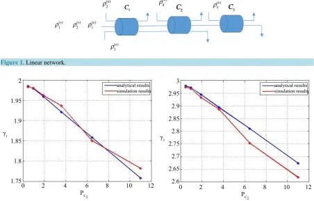
confi-gurations are illustrated in Table 1. Two streaming flow-classes and five elastic flow-classes compete for the resources of the network. Table 2 gives the parameters values of traffic carried by this network.
While C2 is variable, the two other capacities C1 and C3 are fixed in such that PC1=0.47% and 3 0.31%
C
P = .
For this network, we assume that flows with the same maximum bit rate use the same queue, and we assume that for each link l∈:
( ) ( ) ( )
,1 ,2 , l
e e e
l l l M
d ≤d ≤≤d
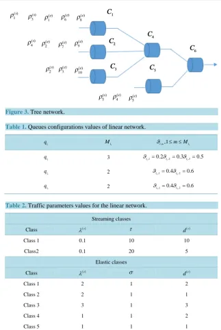
Figure 2 plots a comparison between the analytical results and the simulation results of the average flow throughput as a function of the percentage of PC2 for the first and the third class flows. As expected, the local instability affects badly the average flow throughput for each class. The capacity of links can be then fixed ac-cording to the total load passing through it and the level of QoS that we aim to provide for elastic traffic.
We can note that for values of PC2 inferior to 11%, the two results are very close: the error rate does not ex-ceed 3% for both classes, and it seems a little bit inferior to 1% when PC2 is less than 5%. This observation confirms our results and proves that in a stable system where PC2 remains negligible, our approximation esti-mates very well the performance of the elastic traffic under multi-queuing system.
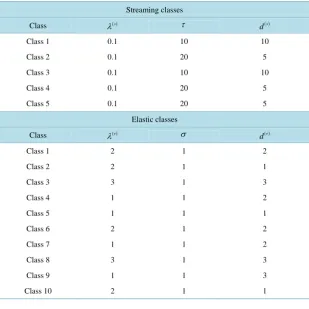
4.2. Tree Network
Now let us consider the tree network illustrated in Figure 3. Five streaming flow-classes and ten elastic flow–classes compete for the resources of the network. Table 3gives the parameters values of traffic crossing this network. All queues are LLQ and their configurations are illustrated in Table 4.
1
C , C2, C3, C4 and C5 are fixed in such that PC1=0.02%, PC2 =0.02%, PC3=0.09%, PC4 =0.06%
[image:11.595.86.539.402.691.2]and PC5 =0.09%. The capacity C6 is variable. For this network, we assume that flows with different maxi-mum bit rate can pass on the same queue. Along its path, each flow passes on queues having the same code
Figure 1. Linear network.
Figure 2. Comparison between the analytical result and the simulation result of the average flow throughput as a function of
Figure 3. Tree network.
Table 1.Queues configurations values of linear network.
i
l
q
i
l
M ϑl m, ,1≤ ≤m Mli
1
l
q 3 ϑl1,1=0.2ϑl1,2=0.3ϑl1,3=0.5
2
l
q 2 ϑl2,1=0.4ϑl2,2=0.6
3
l
q 2 ϑl3,1=0.4ϑl3,2=0.6
Table 2.Traffic parameters values for the linear network.
Streaming classes
Class λ( )s τ ( )s
d
Class 1 0.1 10 10
Class2 0.1 20 5
Elastic classes
Class λ( )e σ ( )e
d
Class 1 2 1 2
Class 2 2 1 1
Class 3 3 1 3
Class 4 1 1 2
Class 5 1 1 1
point. We assume that the flows of class 1, 7 and 10 pass on the queues having a Code Point equal to 20, the flows of class 5, 6 and 9 pass on queues having a Code Point equal to 30 and the rest of class-flows passes on queues having a Code Point equal to 40.
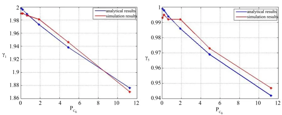
A comparison between the analytical results and the simulation results of the average flow throughput as a function of the percentage of PC6 for the first and the fifth class flows is respectively shown in Figure 4.
In a stable zone, where PC6 is less than 12%, we observe that the relative error is less than 2% for both classes which confirms the good behavior of our approximation.
[image:12.595.157.468.387.562.2]Table 3.Traffic parameters values for the tree network.
Streaming classes
Class λ( )s τ ( )s
d
Class 1 0.1 10 10
Class 2 0.1 20 5
Class 3 0.1 10 10
Class 4 0.1 20 5
Class 5 0.1 20 5
Elastic classes
Class λ( )e σ ( )e
d
Class 1 2 1 2
Class 2 2 1 1
Class 3 3 1 3
Class 4 1 1 2
Class 5 1 1 1
Class 6 2 1 2
Class 7 1 1 2
Class 8 3 1 3
Class 9 1 1 3
Class 10 2 1 1
Table 4. Configurations of LLQ Queues for the tree network.
i
l
q Mli ϑ − −l m, CPl m, ,1≤ ≤m Mli
1
l
q 3 0.2--200.3--30 0.5--40
2
l
q 3 0.2--200.3--30 0.5--40
3
l
q 2 0.4--200.6--40
4
l
q 3 0.2--200.3--30 0.5--40
5
l
q 2 0.4--300.6--40
6
l
q 3 0.2--200.3--30 0.5--40
to be maintained approximately even when accounting for disparities due to packet level behavior [26].
5. Conclusions
Figure 4. Comparison between the analytical results and the simulation results of the average flow throughput as a function of the percentage
2
C
P for the first and the fifth class.
The problem that we studied reflects the reality (and the complexity) of the Internet multimedia processes with heterogeneous flows, differentiated classes of services and different transport protocols. The expression given to evaluate the average end-to-end throughput of elastic traffic under a multi-queuing system using a qua-si-stationary assumption is precise and allows a generalization for large networks with a reasonable computation time.
Another key result is that the approximation proposed is insensitive to detailed traffic characteristics. This is particularly important for data network engineering since performance can be predicted from an estimate of overall traffic volume alone and is independent of changes in the mix of user applications. We expect results such as those presented in this paper to eventually lead to simple and robust traffic engineering rules and per-formance evaluation methods that are lacking for data networks.
References
[1] Boussada, M.E.H., Garcia, J.M. and Frikha, M. (2015) Flow Level Modelling of Internet Traffic in Diffserv Queuing.
Proceedings of the 5th International Conference on Communications and Networking, Hammamet, November 2015.
[2] Garcia, J.M. and Boussada, M.E.H. (2016) Evaluation des performances bout en bout du trafic TCP sous le régime
«Équité Équilibrée». Proceedings of the 11th Performance Evaluation Workshop, Toulouse, March 2016, 15.
[3] Boussada, M.E.L., Garcia, J.M. and Frikha, M. (2016) Evaluation des performances bout en bout du trafic TCP dans
une architecture de réseau multi files d’attente. The 17th Congress of the French Society of Operations Research and
Decision Support (ROADEF), Compiegne, February 2016, 72.
[4] http://www.cisco.com/en/US/tech/tk543/tk544/tk399/tsd_technology_support_sub-protocol_home.html
[5] http://www.enterprise.huawei.comilink/enenterprise/download/HW_U_149185
[6] http://www.journaldunet.com
[7] http://www.e-commercons.com
[8] http://www.lemonde.fr/technologies/article/2012/10/11/2-3-milliards-d-internautes-dans-le-monde_1774055_651865.h tml
[9] Cheikh, H.B. (2015) Evaluation et optimisation de la performance des flots dans les réseaux stochastiques à partage de
bande passante. PhDThesis, INSA, Toulouse.
[10] Olivier, B., Al Sheikh, A. and Garcia, J.M. (2009) Flow-Level Modelling of TCP Traffic Using GPS Queueing
Net-works. 21st International Teletraffic Congress, Paris, 2009, 1-8.
[11] Alexandra Mihaela, N. (2009) Mécanismes d'optimisation multi-niveaux pour IP sur satellites de nouvelle génération.
Diss.
[12] Thomas, B. and Virtamo, J. (2004) Calculating the Flow Level Performance of Balanced Fairness in Tree Networks.
[13] Bertsekas, D. and Gallager, R. (1992) Data Networks. 2nd Edition, Prentice Hall, Englewood Cliffs.
[14] Kelly, F., Mauloo, A. and Tan, D. (1998) Rate Control for Communication Networks: Shadow Prices, Proportional
Fairness and Stability. Journal of the Operational Research Society, 49, 237-252.
http://dx.doi.org/10.1057/palgrave.jors.2600523
[15] Bonald, T., Haddad, J.P. and Mazumdar, R.R. (2011) Congestion in Large Balanced Multirate Links. Proceedings of
the 23rd International Teletraffic Congress, San Francisco, 2011, 182-189.
[16] Bonald, T., Massouli´e, L., Prouti`ere, A. and Virtamo, J. (2006) A Queuing Analysis of Max-Min Fairness,
Propor-tional Fairness and Balanced Fairness. Queueing Systems, Theory and Applications, 53, 65-84.
http://dx.doi.org/10.1007/s11134-006-7587-7
[17] Bonald, T. and Prouti`ere, A. (2003) Insensitive Bandwidth Sharing in Data Networks. Queueing Systems, Theory and
Applications, 44, 69-100. http://dx.doi.org/10.1023/A:1024094807532
[18] Massouli´e, L. (2007) Structural Properties of Proportional Fairness: Stability and Insensitivity. The Annals of Applied
Probability, 17, 809-839. http://dx.doi.org/10.1214/105051606000000907
[19] Bonald, T., Penttinen, A. and Virtamo, J. (2006) On Light and Heavy Traffic Approximations of Balanced Fairness.
2006 ACM SIGMETRICS International Conference on Measurement and Modeling of Computer Systems,Saint Malo,
26-30 June 2006, 109-120. http://dx.doi.org/10.1145/1140103.1140291
[20] Bonald, T. and Proutière, A. (2004) On Performance Bounds for the Integration of Elastic and Adaptive Streaming
Flows. Proceedings of the Joint International Conference on Measurement and Modeling of Computer Systems, New
York, 12-16 June 2004,235-245. http://dx.doi.org/10.1145/1012888.1005716
[21] Delcoigne, F., Proutiere, A. and Régnié, G. (2004) Modeling Integration of Streaming and Data Traffic. Performance
Evaluation, 55, 185-209. http://dx.doi.org/10.1016/S0166-5316(03)00115-9
[22] Key, P., Massoulié, L., Bain, A. and Kelly, F. (2004) Fair Internet Traffic Integration: Network Flow Models and
Analysis. Annals of Telecommunications, 59, 1338-1352.
[23] Queija, R.N., Van den Berg, J.L. and Mandjes, M.R.H. (1999) Performance Evaluation of Strategies for Integration of
Elastic and Stream Traffic.Report-Probability, Networks and Algorithms, No 3, 1-17.
[24] Benameur, N., Fredj, S.B., Delcoigne, F., Oueslati-Boulahia, S. and Roberts, J.W. (2001) Integrated Admission
Con-trol for Streaming and Elastic Traffic. In:Smirnov, M.I., Crowcroft, J., Roberts, J. and Boavida, F., Eds., Quality of
Future Internet Services, Springer, Berlin, 69-81. http://dx.doi.org/10.1007/3-540-45412-8_6
[25] Malhotra, R. and van den Berg, J.L. (2006) Flow Level Performance Approximations for Elastic Traffic Integrated
with Prioritized Stream Traffic. 12th International Telecommunications Network Strategy and Planning Symposium,
New Delhi,November 2006, 1-9. http://dx.doi.org/10.1109/netwks.2006.300367
[26] Thomas, B. and Roberts, J.W. (2003) Congestion at Flow Level and the Impact of User Behaviour. Computer