Reduced Differential Transform Method for Solving Linear and Nonlinear Goursat Problem

(1)

http://dx.doi.org/10.4236/am.2016.710092

Reduced Differential Transform Method

for Solving Linear and Nonlinear Goursat

Problem

Sharaf Mohmoud

1

, Mohamed Gubara

2

1_{Department of Mathematics, College of Science, Omdurman Islamic University, Khartoum, Sudan} 2_{Department of Mathematics, College of Science, AL-Neelain University, Khartoum, Sudan}

Received 12 April 2016; accepted 12 June 2016; published 15 June 2016

This work is licensed under the Creative Commons Attribution International License (CC BY). http://creativecommons.org/licenses/by/4.0/

Abstract

In this paper a new method for solving Goursat problem is introduced using Reduced Differential Transform Method (RDTM). The approximate analytical solution of the problem is calculated in the form of series with easily computable components. The comparison of the methodology pre-sented in this paper with some other well known techniques demonstrates the effectiveness and power of the newly proposed methodology.

Keywords

Reduced Differential Transform Method, Goursat Problem, Adomian Decomposition Method (ADM), Variational Iteration Method (VIM)

1. Introduction

In this paper, we consider the standard form of the Goursat problem [1][2] as provided below

(

, , , ,

)

, 0 , 0

xt x t

u = f x t u u u ≤ ≤x a ≤ ≤t b (1)

( )

, 0

( ) ( ) ( ) ( ) ( ) ( )

, 0, , 0 0 0, 0

u x =g x u t =h t g =h =u (2)

This equation has been examined by several numerical methods such as Runge-Kutta method, finite differ-ence method, finite elements method and Adomian Decomposition Method (ADM).

(2)

lineari-zation, discretization or perturbation.

2. One Dimensional Differential Transform Method

The differential transform of the function w x

( )

is defined as follows

( )

0 d 1 ! d k k x w x W k

k x ₌

 

 

 

= (3)

where w x

( )

is the original function and W k

( )

is the transformed function. Here d d

k

x means the k

th deriv-

ative with respect to x.

The differential inverse transform of W k

( )

is defined as

( )

0

k

w x W k x

∞

=

∑

(4)

Combining (3) and (4) yields

( )

0 d 1 ! d k k k k w x

w x x

k x ∞ =   =      

∑

(5)

From (3) and (4) it is easy to see that the concept of the differential transform is derived from Taylor series expansion [see Table 1].

3. Analysis of the Reduced Differential Transform Method

The basic definitions of reduced differential transform method are introduced below. Definition

Assume that the function u x t

( )

, is analytic and continuously differentiable with respect to time t and space x in the domain of interest, then let

( )

0 d , 1 ! d k k k t

u x t

U x

k t ₌

 

=  

 

  (6)

Where the t-dimensional spectrum function U_k

( )

x is the transformed function. The differential inverse of

( )

k

U x is defined as follows

( )

0

, k

k k

u x t U x t

∞

=

∑

(7)

Then combining Equation (6) and (7) we can write

( )

0 0 d , 1 , ! d k k k k t

u x t

u x t t

k t ∞ = ₌   =      

[image:2.595.82.541.91.327.2]

∑

(8)

Table 1. One-dimensional differential transformation [3].

Function form Transformed form

( ) ( )

u x ±v x U k

( ) ( )

±V k

( )

cu x cU K

( )

d d m m u x x

(

_{) ( )}

! ! k m

U k m

k

+

( ) ( ) ( )

w x =u x +v x

( )

( ) (

)

0

k

r

W k U r V k r

=

(3)

Now, we express the Goursat problem in the standard operator form.

( )

(

,

)

(

( )

,

)

R u x t =L u x t (9)

With the initial conditions

( )

, 0

( ) ( ) ( )

, 0, , and

( ) ( ) ( )

0 0 0, 0

u x =g x u t =h t g =h =u (10)

where

( )

(

,

)

_xt

( )

, and

(

( )

,

)

(

, , , _x, _t

)

R u x t =u x t L u x t = f x t u u u

We applying RDTM of Equations (1) and (2) giving

( )

(

_xt ,

)

(

, , , _x, _t

)

RDT u x t =RDT f x t u u u (11)

( )

(

, 0

)

RDT u x =g x (12)

(

k+1

)

Uk+1

( )

x =FK

( )

x (13)

( )

( ) ( )

0

U x = g x δ k (14)

where F_K

( )

x is transformed value of f x t u u u

(

, , , x, t

)

and g x

( ) ( )

δ k is transformed value of u x

( )

, 0 . By iterative calculations we obtain the following values of U_k

( )

x as:

( )

( ) ( )

( )

1 1 , 2 2 , 3 3 , , n n

U x =ρ x U x =ρ x U x =ρ x U x =ρ x (15)

From (7) we have.

( )

0

( )

1

( )

2

( )

0 1 2

, n

n

u x t =U x t +U x t +U x t + + U x t (16)

One can get the exact solution of (1) by substituting (14) and (15) in (16).

[image:3.595.187.440.450.720.2]

With reference to the articles [4][5]. We easy prove the transformation in the following Table 2.

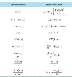
Table 2.Reduced differential transformation.

Functional form Transformed form

( )

,

u x t

( )

0

d ,

1

! d

k

K k

t u x t

U x

k t

=

 

 

 

=

( ) ( )

, ,

u x t ±v x t Uk

( )

x ±V xk

( )

, u x t

∝ ∝Uk

( ) (

x ∝is a constant

)

m n

x t xmδ

(

k−n

)

( )

, m n

x t u x t m

(

)

x U k−n

( ) ( )

, ,

u x t v x t

( ) ( )

0

k

r k r r

U x V− x

=

∑

( )

d ,

d r

r u x t

t

(

)

!

_{( )}

! k r

k r

U x

k +

+

( )

d ,

d u x t

x

( )

d

d k

U x

x

( )

d ,

d d r s

r s u x t

x t

+

(

)

d

( )

d k s

r

U x

k s

x

+

(4)

4. Application and Results

In this section, we apply the method to some linear and non linear Goursat problem in order to demonstrate its efficiency.

A.The linear homogeneousGoursat problem

We first consider the linear homogeneous Goursat problem defined below

( )

,

(

( )

,

)

xt

u x t =L u x t (17)

( )

, 0

( ) ( ) ( )

, 0, and

( ) ( ) ( )

0 0 0, 0

u x =g x u t =h t g =h =u (18)

Where L u x t

(

( )

,

)

is a linear function of u.

Example 1: Consider the homogeneous Goursat problem

xt

u =u (19)

( )

, 0 e ,x

( )

0, e ,t

( )

0, 0 1

u x = u t = u = (20)

Taking RDTM of (19) and (20), we obtain

(

)

1

d 1

d k k

k U U

x +

+ = (21)

0 e

x

U = (22)

Substituting (22) into (21) and using the recurrence relation, we will reach to the results listed below.

1 2 3 4

e e e

e , , , ,

2 3! 4!

x x x

x

U = U = U = U = 

And so on. In general, we have e ! x

K

U k

= for

k

=

1, 2,



substituting all U_k into (7) yields the solution

( )

, ex t

u x t = + . This result is in full agreement with the one obtained in [6] by VIM. Example 2: Now consider the homogeneous Goursat problem

2 xt

u = − u (23)

( )

, 0 e ,x

( )

0, e ,t

( )

0, 0 1

u x = u t = u = (24)

Applying RDT to (23) and (24) we obtain

(

)

1

d

1 2

d k k

k U U

x +

+ = − (25)

0 e

x

U = (26)

Substituting (26) into (25) and using the recurrence relation we have

1 2 3 4

4 2

2e , 2e , e , e

3 3 ,

x x x x

U = − U = U =− U = 

And so on. By substituting all U_k into (7), the solution becomes

( )

, ex 2t

u x t = − . This results perfectly matches the results obtained in [6] by VIM.

B. The linear inhomogeneousGoursat problem: We now consider inhomogeneous Goursat problem

( )

, xt

u =L u +w x t

( )

, 0

( ) ( ) ( ) ( )

, 0, , 0, 0

( ) ( )

0 0

u x =g x u t =h t u =g =h

where L u

( )

is linear function of u.

(5)

xt

u = −u t (27)

( )

, 0 e ,x

( )

0, e ,t

( )

0, 0 1

u x = u t = +t u = (28)

Taking RDM of (27) and (28) will lead to

(

)

1

( )

d 1

d k k

k U U t k

t + δ

+ = − (29)

0 e

t

U = +t (30)

1 2 3 4

e e e

e , , , ,

2 3! 4!

t t t

t

U = U = U = U = 

k

U k

= for

k

=

1, 2,



substituting all U_k in (7) yields the solution

( )

, ex t

u x t = +t + , this result is again identical to the one obtained in [6] by VIM . Example 4: Consider the linear in homogeneous Goursat problem

2 2 4 xt

u = +u xt−x t (31)

( )

, 0 e ,x

( )

0, e ,t

( )

0, 0 1

u x = u t = u = (32)

Taking RDM of (31) and (32) gives rise to

(

)

(

)

2

(

)

1

d

1 4 1 2

d k k

k U U x k x k

x + δ δ

+ = + − − − (33)

0 e

x

U = (34)

2

1 2 3 4

e e e

e , , , ,

2 3! 4!

t t t

x

U = U = +x U = U = 

k

U k

= except 2

2

e 2

x

U = +x substituting all U_k in (7) yields the solu-

tion

( )

, 2 2 ex t

u x t =x t + + , This result is again in full agreement with one obtained in [6] by VIM . C. The non-linear Goursat problem:

( )

, n

( )

,

xt

u = f x t +u x t (35)

( )

, 0

( ) ( ) ( ) ( )

, 0, , 0, 0

( ) ( )

0 0

u x =g x u t =h t u =g =h (36)

where

( )

,

n

u x t is non-linear term.

Here, we apply RDTM to non-linear Goursat problem. Example 5: We first consider the non-linear Goursat problem .

3 2 2 3

3 3

xt

u = − +u x + x t+ xt +t (37)

( )

, 0 ,

( )

0, ,

( )

0, 0 0

u x =x u t =t u = (38)

Taking RDM of (37), (38) yields

(

)

2 3

( )

2

(

)

(

) (

)

1 0 d

1 3 1 3 2 3

d

k

k r k r

r

k U u u x k x k x k k

x + = − δ δ δ δ

+ = −

∑

+ + − + − + − (39)

And

0 r

r s r s s

U U U −

=

(6)

0

U =x (41)

Substituting (41) into (40) and (39) and using the recurrence relation we have

1 1, and 2 3 4 5 n 0

U = U =U =U =U ==U = yields the solution u x t

( )

, = +x t which is in full agreement with one obtained in [6] by VIM.

Example 6: We finally consider the non-linear Goursat problem

2 e u xt

u = − (42)

( )

, 0 0,

( )

0, 0,

( )

0, 0 0

u x = u t = u = (43)

Taking RDM of (42) and (43) we obtain

(

)

1

( )

d 1

d k k k

k U N U

x +

+ = (44)

where N U

( )

_K is the reduced transform of 2 e−u

such that 0 e2 0, 1 2e2 0 1

U U

N = − N = − − U

And so on,

0 0

U = (45)

2 3

1 , and 2 , 3 ,

2 3

x x

U =x U = − U =  and

so on.

Therefore, the solution is u x t

( )

, =ln 1

(

+xt

)

which is the exact solution.

5. Comparison

In this section, we use the Adomian decomposition method to obtain the solution of (1) and (2). and discuss the comparison between the reduced differential transform method and the Adomian decomposition method.

With reference to the article [7]-[9], (1) can be rewritten In an operator form as:

(

, , , ,

)

x t x t

l l u= f x t u u u (46)

where

d d

,

d d

x t

l l

x t

= = (47)

The inverse operators l_x−1 and l_t−1 can defined as:

( ) ( )

1 1

0 0

. . d , . . d

x t

l− =

∫

x l− =

∫

t (48)

By applying l_x−1 and l_t−1 respectively to both sides of (46) and substituting

( )

0

, _n ,

n

u x t =

∑

∞₌ u x t gives

( )

( ) ( ) ( )

1 1

(

)

0

, 0 , , , ,

n x t x t

n

u x t g x h t g l l f x t u u u

∞

− −

=

= + − +

∑

(49)

Adomian method admits the use of recursive relation

( )

0 , ,

u x t =

ρ

x t (50)

( )

1 1

(

)

1 , , _x, _t 0

k x t k k k

u₊ x t =l l− −σ u u u k≥ (51)

where

( )

( ) ( ) ( )

(

)

( ) ( ) ( )

1 1

( )

(

)

0 , , ,

,

0 , , , ,

x t

x t x t

g x h t g f u u u

x t

g x h t g l l x t f x t u u u

σ ρ

τ τ σ

− −

 + − =

 = 

+ − + = +

 (52)

(7)

Following the pervious discussion and using (49) Equations (27) and (28) gives

( )

2 1 1

( )

0 0

1

, e e 1 ,

2 x t

n x t n

n n

u x t x x t l l u x t

∞ ∞

− −

= =

 

= + + − − + _ _

 

∑

(53)

This gives

( )

, ex t

u x t = +x + (54)

This result is again identical to the one obtained by the RDTM example (3). Again applying pervious discussion and using (49) Equations (42) and (43) gives

( )

1 1

0 0

,

n x t n

n n

u x t l l A

∞ ∞

− −

= =

 

= _ _

 

∑

(55)

where A_n are adomian polynomials for the nonlinear term e−2u giving by

(

)

0 0 0

2 2 2 2

0 e , 1 2 e1 , 2 4 1 2 2 e ,

u u u

A = − A = − u − A = u − u − 

Then the closed form solution is giving by

( )

, ln 1

(

)

u x t = +xt (56)

This result is again identical to the one obtained by RDTM in example (6).

We have carried out the comparative study between the reduced differential transform method and the Ado-mian decomposition method by handling the Goursat problem, Two numerical examples have shown that the reduced differential transform method is a very simple technique to handle linear and nonlinear Goursat problem than the Adomian decomposition method, and also, it is demonstrated that the reduced differential transform method solves linear and nonlinear Goursat problem without using any complicated polynomials like as the Adomian polynomials.

In addition, the obtained series solution by the reduced differential transform method converges faster than those obtained by the Adomian decomposition method. It is concluded that this simple reduced differential transform method is a powerful technique to handle linear and nonlinear initial value problems.

6. Conclusion

The Goursat problem has been analyzed using reduced differential transform method. All the illustrative exam-ples have shown that the reduced differential transform method is powerful mathematical tool to solving Goursat problem. It is also a promising method to solve other nonlinear equations, the presented method reduces the computational difficulties existing in the other traditional methods and all the calculations can be done by simple manipulations.

References

[1] Zhou, J.K. (1986) Differential Transform and Its Applications for Electrical Circuits. Huazhong University Press, Wu-han.

[2] Wazwaz, A.M. (1993) On the Numerical Solution of the Goursat Problem. Applied Mathematics and Computation, 59, 89-95. http://dx.doi.org/10.1016/0096-3003(93)90036-e

[3] Keskin, Y., Caglar, I. and Koc, A.B. (2011) Numaerical Solution of Sine-Gordon Equation by Reduced Differential Transform Method. WEC, 1, 6-8.

[4] Day, J.T. (1966) A Runge-Kutta Method for the Numerical Solution of the Goursat Problem in Hyperbolic Partial Dif-ferential Equations. The Computer Journal, 9, 81-83. http://dx.doi.org/10.1093/comjnl/9.1.81

[5] Evans, D.J. and Sanugi, B.B. (1988) Numerical Solution of the Goursat Problem by a Nonlinear Trapezoidal Formula. Applied Mathematics Letters, 1, 221-223. http://dx.doi.org/10.1016/0893-9659(88)90080-8

[6] Wazwaz, A.M. (2007) The Variational Iteration Method for a Reliable Treatment of the Linear and the Nonlinear Goursat Problem. Applied Mathematics and Computation, 193, 455-462. http://dx.doi.org/10.1016/j.amc.2007.03.083

(8)

[8] Wazwaz, A.M. (2002) Partial Differential Equations: Methods and Applications. Balkema Publishers, The Nether-lands.