What is the Shape of Real Exchange Rate Nonlinearity?

Munich Personal RePEc Archive

What is the Shape of Real Exchange

Rate Nonlinearity?

Norman, Stephen and Phillips, Kerk L.

University of Washington, Tacoma, Brigham Young University

May 2009

Online at

https://mpra.ub.uni-muenchen.de/23504/

What is the Shape of Real Exchange Rate Nonlinearity?

Stephen Norman

University of Washington, Tacoma

Kerk Phillips

Brigham Young University

May 7, 2009

Abstract

Evidence that real exchange rate dynamics can be described using models which ex-hibit nonlinear mean reversion has been mounting over the past several years. This pa-per attempts to better understand the shape of real exchange rate nonlinearity through the use of the smooth transition autoregressive (STAR) model and the newly proposed skewed generalized error (SGE) transition function. The advantage of this transition function is that is nests popularly used transition functions through simple parameter constraints. This allows the use of nested model selection tests. It is shown that more flexible transition functions are preferred in many cases over the commonly used ex-ponential transition function. The results suggest that most of the real exchange rates studied in this paper are better described by discrete threshold models rather than STAR models.

∗_{Email: [email protected]; University of Washington - Tacoma, 1900 Commerce St, Campus}

Box 358420, Tacoma WA 98402-3100; Tel: 253-692-4827

1

Introduction

Purchasing power parity (PPP) states that a basket of goods should have the same price

in any country when prices are expressed in a common currency. One common method

of seeking evidence for the existence of PPP is to test for long run mean reversion in real

exchange rates. Taylor, Peel, and Sarno (2001) cite two puzzles related to purchasing power

parity. The first is the difficulty of rejecting the presence of a unit root in real exchange rates

using conventional tests based on linear models. The second is the consensus (see Rogoff

(1996)) that, even when evidence of mean reversion can be found, real exchange rates revert

very slowly to the long run mean with half lives on the order of 3-5 years.

Over the past several years, nonlinear mean reversion in real exchange rates has received

much attention because it is one possible solution to these two PPP puzzles. The economic

theory which motivates this approach has its beginnings with Heckscher (1916) who

hypoth-esized that adjustment towards the law of one price (LOOP) should not take place if price

differentials in international goods markets were small. This is due to the fact that

trans-portation costs and other impediments to trade render arbitrage unprofitable if the possible

revenue from committing arbitrage is smaller than the associated costs. Small deviations

from LOOP are then persistent given the absence of arbitrage. Only when differences in

prices are sufficiently large is arbitrage profitable. Thus the theory of international goods

market arbitrage in the presence of trade frictions implies that the speed of mean reversion

in relative prices should vary depending on how far relative prices are from their equilibrium

value.

Discrete threshold autoregressive (TAR) models have been used to model the dynamics of

relative prices of individual goods.1

When working with relative prices based upon a basket

1

of goods with varying transportation costs and trade impediments, as is the case with real

exchange rates, intuition suggests that the transition should be smooth rather than discrete.

This has led to the wide use of the smooth transition autoregressive (STAR) model. This

model describes the data in terms of different regimes where the transition from one regime

is governed by the transition function,R(zt, θ), which is a smooth function bounded between zero and one, R :R→ [0,1]. In the context of PPP, many empirical applications using the STAR model employ two regimes. One regime represents the unit root behavior of the real

exchange rate when it is near its long run equilibrium, and the other regime models mean

reversion which should be observed when the exchange rate is far from its mean.

One simple STAR model that could be used in this context is:

yt−µ=ρ1(yt−1−µ) + (ρ2−ρ1)(yt−1−µ)R(zt, θ) +εt (1)

whereytis the real exchange rate at timetand µis the long run equilibrium. If the theory of international arbitrage in the presence of transportation costs holds, one would expect that

ρ1 = 1 and ρ2 < 1. The transition function would also need to be an inversely bell-shaped

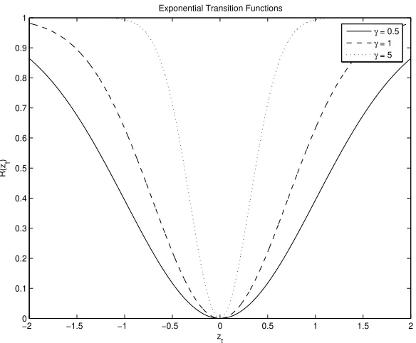
function that is bounded between one and zero. The exponential function,

R(zt;µ, γ) = 1₋exp[₋γ(zt−µ)

2

], (2)

is the most popular transition function used to model nonlinear mean reversion in the context

of PPP. This function has two limitations. The first is that it is constrained to be symmetric

about the parameter µ. This implies the rate of mean reversion of the exchange rate will be the same whether the exchange rate is greater than its mean or an equal distance below

its mean. There has been recent evidence that mean reversion may not be symmetric.2

The

2

second limitation which was identified by Bec, Ben Salem, and Carrasco (2004), stems from

fact that “neither the discontinuous nor the continuous adjustment cases can be ruled out

a priori on theoretical grounds.” In other words, it would be desirable to use a transition

function that could model both continuous and discrete adjustments in the speed of mean

reversion.

A major contribution of this paper is the introduction of a flexible transition function

which we call the skewed generalized error (SGE) transition function after the skewed

gen-eralized error distribution on which it is based. While other transition functions have been

suggested that can model asymmetric mean reversion and near discrete transitions, the SGE

transition function’s advantages over alternatives include: greater ease of estimation and

interpretation, the ability to model a wider range of possible shapes, and the fact that it

directly nests the exponential transition function and the TAR model. This last advantage

implies conventional model selection tests can be used instead of non-nested model selection

tests to determine if this new transition function is preferred over the popular exponential

transition function.

The results in this paper provide evidence of nonlinear mean reversion with TAR-like

dynamics and/or asymmetries is almost all real exchange rates examined. Discrete thresholds

appear to be a better description of the time-series dynamics that the smoother transitions

imposed by ESTAR models. This is counter-intuitive if the primary force driving mean

reversion is arbitrage behavior. However, it is consistent with the notion that central banks

intervene to push real exchange rates back toward PPP whenever they deviate too far. The

remainder of the paper is as follows. In section two, flexible transition functions are discussed.

2

Flexible Transition Functions

A two regime STAR model can be expressed in the following manner:

yt= (α0 +α1yt−1 +. . .+αpyt−p)

+ [(β0−α0) + (β1−α1)yt−1 +. . .+ (βp−αp)yt−p]R(zt, θ) +εt, (3)

or equivalently

yt =α′xt+ (β′ −α′)xtR(zt, θ) +εt, (4)

where xt = (1, yt−1, . . . , yt−p)′, α = (α0, α1, . . . , αp)′, and β = (β0, β1, . . . , βp)′. Whether the

time series process follows a AR(p) model parameterized byα,β, or some convex combination of the two regimes is governed by the transition function R(_·), which is a function of some transition variable zt and a set of parameters θ. In the STAR model, R(zt, θ) is a smooth function bounded between zero and one,R :R→[0,1]. The value of the transition function determines the proportion of each regime present in the dynamics of the process depending

on the value of the transition variable.

It is useful to note that the well used exponential transition function in (2) has the same

functional form as the Gaussian PDF without the normalizing constant. This connection

between the exponential transition function and the normal distribution suggests that

alter-native transition functions could be found by taking some other PDF, sayf(_·), and using as the transition function, 1₋cf(x), where cis any constant such that max

x {1−cf(x)}= 1.

The exponential transition function has at least two limitations. First, it has a constant

“peakedness” in the sense that Gaussian distribution has a constant kurtosis regardless of

the mean or variance. It might be desirable to have a transition function which can take

would be based on PDF with a smaller kurtosis than the Gaussian distribution. The second

limitation of the exponential transition function is that it is symmetric. It is possible that

the nonlinear mean reversion might be asymmetric around the mean.

One distribution that allows for both of the above modifications, is the skewed

general-ized error (SGE) distribution (see Hansen, McDonald, and Theodossiou, 2007). The SGE

distribution is defined by

f(x;µ, σ, α, φ) = φ

2σΓ(1/α)exp

−

|x₋µ_|

(1 + sign(x₋µ)φ)σ

α

, (5)

where _−∞ < µ < +_∞ and σ > 0 are the location and scale parameters, α > 0 controls the kurtosis, and ₋1 < φ < 1 determines the skewness. The distribution is symmetric for

φ= 0, positively skewed for φ >0, and negatively skewed for φ <0. As α_→0 the kurtosis approaches infinity and as α _{→ ∞} the kurtosis approaches 1.8 (which is the kurtosis of the uniform distribution). Thus the SGE distribution nests the uniform distribution in the limit

and has no upper bound on its kurtosis. The corresponding transition function is:

SGE(zt;µ, γ, α, φ) = 1₋exp

−

|zt−µ|

γ(1 + sign(zt−µ)φ)

α

(6)

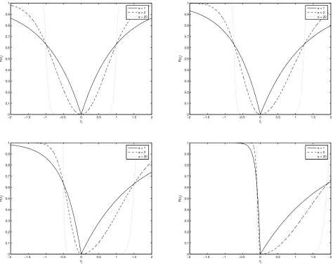
Note that with α = 2 and φ = 0 the SGE transition function represents the exponential transition function. Sample SGE transition functions are plotted in figures ?? - ?? for

parameterizations µ= 0, γ = 1, α = (1,2,20), φ= (0,0.25,0.5,0.9).

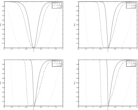
An alterative transition function that can both model asymmetry and nests the TAR

model in the limit was proposed by Siliverstovs (2005). This bi-parameter (BP) STAR

model has the following transition function,

BP(yt−d;γ1, γ2, λ1, λ2) =

exp[₋γ1(yt−d−λ1)] + exp[γ2(yt−d−λ2)]

where γ1 > 0, γ2 > 0, λ1 ≤ λ2. Sample BP transition functions are plotted in figures

?? - ?? for parameterizations µ = 0, γ1 = 5, γ2 = (5,15,25,50), λ1 = (0,−0.5,−1.5),

λ2 = (0,0.5,1.5).3 To compare the SGE and BP transition function, one can construct a

PDF based upon the BP transition function for special case whereγ1 =γ2 andλ1 =λ2 = 0:

P(x;γ) = 3

√

3γ

2π

1₋ exp[−γx] + exp[γx] 1 + exp[₋γx] + exp[γx]

. (8)

Note that the constraint γ1 = γ2 implies symmetry and λ1 = λ2 = 0 produces the highest

possible kurtosis given symmetry. The kurtosis of the PDF represented by (8) is 4.5 for all

values ofγ, while the SGE distribution has no upper limit on the value of its kurtosis in the symmetric case. This is one example of the greater flexibility of the SGE transition function

compared with the BP transition function.

Another drawback of the BP transition function is that the value of transition variable

which yields the minimum value of the transition function, zmin

t , is not directly estimated, it is a nonlinear function of γ1, γ2, λ1, and λ2:

ztmin =

γ1λ1+γ2λ2+ log(γ1/γ2)

γ1+γ2

(9)

With the SGE transition function it follows thatzmin

t =µ. In the context of nonlinear mean reversion, the minimum of the transition function represents the mean of the process. This

implies that any restriction made on the mean with the BP transition function will require

a nonlinear constraint. For example in the following specification that is used in this paper,

yt−m= [α1(yt−1−m) +. . .+αp(yt−p−m)][1−R(yt−d;θ)] +εt. (10)

with the SGE transition function it is simple make the constraint that zmin

t =m by setting

3

m = µ. Making the same constraint with the BP transition function requires a nonlinear constraint.

One advantage of the BP transition function is that for λ1 6= λ2 as γ1, γ2 → ∞ the

parameters λ1, and λ2 represent the discrete thresholds. With the SGE transition function

the analogous discrete thresholds are not directly estimated. As α _{→ ∞} the change points are equal to [µ+γ(1+φ), µ₋γ(1₋φ)]. Thus, the implied thresholds are easily computed given the parameter estimates of the transition function. While it is true that any restrictions made

on the discrete thresholds would necessitate a nonlinear constraint with the SGE transition

functions, such restrictions are rarely made. Discrete thresholds are usually endogenously

chosen.

The fact that two parameter constraints, α = 2, and φ = 0, produce the well used exponential transition function is perhaps its chief advantage in the context of this paper.

When using the SGE transition function one and use nested model selection criterion to

gauge whether the exponential transition function is adequate or if a more flexible transition

function is preferred. Comparing the BP and the exponential transition function would

require the use of non-nested model selection test. Judge et al. (1985 pg. 889) write, “When

we leave the nested model case, the problem becomes more difficult and the results perhaps

a bit more shaky.”

Bec et al. (2004) use a multi-regime logistic STAR model (MR-LSTAR) to model the

dynamics of multiple real exchange rates. Like this paper, they also find evidence of TAR

like dynamics. The MR-LSTAR model allows for both discrete and smooth mean reversion

like the BP and SGE transition functions, but it has the same drawbacks when compared

with using the SGE transition function that the BP STAR model does. Namely it is not

long run mean in the transition function, and it does not directly nest the ESTAR model.

In addition, the MR-LSTAR model does not allow for asymmetric mean reversion. Given

the advantages of the SGE transition function compared with the alternative transition

functions, this paper exclusively uses the SGE transition function.

3

Empirical Application

3.1

Model and Estimation

The STAR models used in this paper are represented by

∆yt=ρ1(yt−1 −µ) +ρ2(yt−1−µ)R(yt−d;θ) +

p

X

i=1

ai∆yt−i+εt (11)

where R(yt−d;θ) is given in (6). Note that with the above SGE-STAR model the mean, µ,

enters into both the autoregressive portion of the model and also the transition function.

If the BP transition function were used, a comparable model would require a nonlinear

constraint. This is a Dicky-Fuller representation of (1) with p augmentation terms. The modeling procedure begins by using Akaike information criterion to choose the number of

lags, p, in a linear version of (11). The transition variable is selected by estimating the following regression equation

∆yt=α0+

N

X

j=1

(αjyjt−d+φjyt−1yj_t−d) +

p

X

i=1

with N = 4 for d = 1, ...,12, and choosing the one which has the smallest sum of squared error.4

This follows the approach of Hansen (1997) who suggests selecting the transition

variable,yt−d, that minimizes the sum of squared errors based on an estimated TAR model.

This paper uses a relatively new test developed by Park and Shintani (2005) which is

de-signed to detect the presence of a unit root against the alternative of stationary transitional

autoregressive models. The inf-t test based on both the ESTAR and D-LSTAR5

transition

functions is employed in an attempt to reject the null of nonstationarity in the real exchange

rates studied in this paper in favor of a stationary STAR model. The STAR model with p

lags andyt−d as the transition variable is then estimated using maximum likelihood.

To facilitate the estimation of the STAR models Leybourne, Newbold, and Vougas (1998)

propose concentrating the sum of squares function. With the general STAR model in (3), for

given values of the parameters in the vector θ the model is linear and can be estimated by ordinary least squares. Thus ifθ is a k_×1 vector of parameters, starting values for the NLS estimation can be found through a k dimension grid search. To reduce the dimensionality of the grid search over the parameters in the transition functionsµwill be set to the sample mean ofyt, ¯y. The possible reduction in the dimension of the grid search is another advantage of the SGE transition function over BP. The grid search used in the estimation process is

further discussed in the appendix.

In an attempt to minimize the possibility of choosing starting values for the ESTAR

nonlinear estimation that were within a local minimum, a grid search was performed not

only for γ, but also for ρ1, ρ2. The grid for the autoregressive parameters was constructed

by choosing ρ1,i ∈ [−1,0] where the interval is divided into 100 equally spaced intervals.

4

The regression in (12) is based upon the true regression model in (11) where the transition function has been replaced by a fourth order Taylor approximation. This will allow the selection of the delay parameter to be based on upon a flexible nonlinear model.

5

The second autoregressive parameter, ρ2,i, is chosen within [−1, ρ1,i] within the same grid.

Inspection of the ESTAR transition function showed that changes inγ had a relatively large impact on the shape of the function when γ was small compared with cases when γ was large. Consequentially, the grid search forγ was constructed in the following manner. In the interval [-5,10], 100 equally spaced numbers were obtained, gi ∈ [−5,10] for i = 1, . . . ,100. The resulting grid was [exp(g1), . . . ,exp(g100)] = [0.01, . . . ,22026.47]. This grid is more

densely concentrated for smaller values of γ.

The behavior the SGE transition function with respect to changes in γ and α followed a similar pattern when compared with the ESTAR model. The grid for γ was constructed in the same manner as γ in the ESTAR model. The grid search for α was constructed by taking 100 equally spaced intervals in [-1,5], ai ∈ [−1,5] for i = 1, . . . ,100, and using as a grid [exp(a1), . . . ,exp(a100)] = [0.37, . . . ,148.41]. The grid search for φ included the 100

equally spaced numbers in (-1,1).

3.2

Data

Data on real exchange rates were obtained for 10 country pairs from the International

Mone-tary Fund’s International Financial Statistics online database. The countries include France

(FR), Germany (GR), Italy (IT), UK, and USA (US). Monthly observations were obtained

from 1973:1 to 1998:1 for France, Germany, Italy, and 1973:1 to 2004:12 for UK and USA.

The real exchange rates (yt) were calculated according to

yt≡st+pt−p∗t,

wherest is the logarithm of the nominal exchange rate (foreign price of domestic currency),

foreign consumer price level. The data was obtained from the International Monetary Fund’s

International Financial Statistics database.

3.3

Results

Table 1 contains the results of augmented Dickey-Fuller unit root tests with and without

a trend. The null of a unit root is rejected at the 5% level for only FR/GR, suggesting

that almost all of the time series may be nonstationary. The LM tests for the presence of

heteroskedasticity is applied to each real exchange rate at lag lengths 1, 6, and 12. FR/UK,

FR/US, and IT/US are the only country pairs that show no evidence of heteroskedasticity.

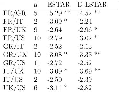
The results of the Park and Shintani (2005) nonlinear unit root tests are found in Table

2. The nonlinear unit root tests are able to reject the presence of a unit root in favor of a

stationary STAR model for the following country pairs: FR/GR, FR/IT, FR/UK, FR/US,

GR/UK, IT/UK, and UK/US at the 5% or 10% significance level. These seven country pairs

are the focus of the remainder of the empirical analysis.

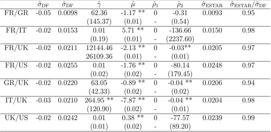
Because the nonlinear model is based on a Dickey-Fuller (DF) model, the results from the

DF regression are used as a baseline and are found in Table 3. Both the DF autoregressive

coefficient and standard error of the regression are reported. The ESTAR model in (11) with

transition function represented by (2) were estimated, and the results are also reported in

Table 3. It has been documented that when estimating two regime ESTAR models it is often

difficult to estimate γ, ρ1, and ρ2 jointly. To facilitate estimation, the following constraints

were used: ρ1 ≤ 0 and ρ2 ≤ ρ2. These constraints eliminate the possibility of explosive

behavior and imply that the rate of mean reversion cannot decrease the further the process

is from its long run equilibrium. The last column in Table 3 shows percent difference in the

model. In all cases there is a reduction in the size of the estimated standard error of the

residual. The maximum reduction is 5% in the case of FR/GR and the minimum is 1% in

the case of UK/US.

The estimation results of the SGE STAR model are found in Table 4. The two parameters

of interest are α and φ. The value of α is very large for all real exchange rates with implies TAR like behavior of the transition functinon. Because the estimated values ofαare so large, this should also cast some doubt upon precision of the estimates of α. This is because for large values of α, the transition function is nearly identical to a discrete threshold transition function. Consequently, changes in α in such cases will have little effect on the fit of the overall model. With respect to asymmetry, ˆφ is statistically different from zero for all countries except for UK/US. Thus in every case the estimated SGE transition function is

nearly discrete even when the model is capable of assuming a exponential transition function

shape. This result is in line with the results of Bec et al. (2004) who also found evidence of

threshold behavior in real exchange rates. The last column in Table 4 again shows percent

difference in the estimated standard error of the residual of the ESTAR model compared

with the SGE model. The reductions in the standard error of the estimated model are

more modest that the comparison of the ESTAR model to the linear model. The maximum

reduction is about 2% in the case of FR/GR, FR/IT, and UK/US data. There is almost no

reduction in the case of FR/UK.

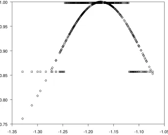
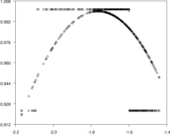
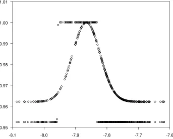
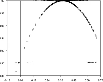
To help visualize the difference between the estimated shape of the nonlinearity in the

ESTAR and SGE models, the values of 1 +ρ1+ρ2R(yt−d;θ) are plotted vs. yt−d in figures 4 to 10. We call this the autoregressive function of the model. It shows the varying degrees of

mean reversion in the model. While the shape of the transition functions are dramatically

different, there is less difference in the rates of mean reversion. To see if there is a statistical

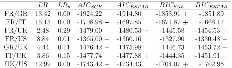
2, φ= 0. Because the ESTAR model is nested in the SGE model a simple likelihood ratio test can be used. Table 5 contains the results of the likelihood ratio test. In three cases the null

hypothesis is not rejected at the 10% significance level: FR/UK, GR/UK, and IT/UK. Thus

for four out of the seven exchange rates, we reject the ESTAR model in favor of the SGE

model. The AIC suggests that the SGE is preferred over the exponential transition function

in all cases except for FR/UK and IT/UK. The BIC, which favors more parsimonious models,

implies the SGE is the preferable model for FR/GR, FR/IT, and UK/US. These results are

in line with the reduction in the standard error of the model found in Table 4.

To further illustrate the how the SGE model is preferred over the ESTAR model, the sum

of squared errors which resulted from the SGE model grid search used to obtain starting

values for the real exchange rate are plotted in Figures 11 to 17 for all combinations of

γ and φ considered. Darker shades correspond to a lower value of the sum of squared errors. For large values of α, the horizontal bands at different values of γ correspond to transition functions that are very close to a discrete threshold transition function. Each

band corresponds to a different threshold value. The left section of the grid search figures

then corresponds to TAR-like models. The right section corresponds to more exponential

like transition functions. ESTAR models would be located along the vertical line were

α = 2. For most of the countries, grid search suggests that transition functions similar to discrete threshold transition functions seem to fit the data best. The most notable exception

is FR/UK where there is a local minimum in the sum of squares function where α = 2. FR/UK is also the real exchange rate that showed the least difference between the ESTAR

4

Conclusion

This paper has introduced and estimated a very general functional form the transition

func-tion of the STAR model. The SGE funcfunc-tion we use nests both the exponential STAR model

and a threshold model as special cases. Our estimation shows that the majority the real

exchange rate series we examine are best described by the threshold model rather than the

ESTAR model. Our results indicate that ESTAR models misspecify the time-series behavior

of real exchange rates by imposing smooth transitions between high and low persistence

regimes that are not justified by the data.

There is a great deal of intuitive appeal to the some sort of smoothed transition in real

exchange rates. Arbitrage opportunities are thought drive long-run convergence to PPP

and underlie mean reversion in real exchange rates. These must apply to different goods at

different deviations from PPP due to wide disparities in transportation costs among other

reasons. This implies that pressure to revert to the mean will gradually build up as the

real exchange rate deviates further and further from PPP, exactly what the ESTAR model

allows.

Our estimation strongly rejects this formulation, however, in favor of thresholds in

re-version. Inside a band in the neighborhood of PPP, the real exchange rate follows a process

that is close to a random walk. Outside the neighborhood of PPP, however, the rate quickly

reverts back to the band. This type of behavior is consistent with real exchange rates being

held inside bands by the actions of central banks through short-run manipulation of nominal

References

Bec, F., M. Ben Salem, and M. Carrasco (2004): “Detecting mean reversion in real

ex-change rates from a multiple regime star model,” RCER Working Papers 509, University

of Rochester - Center for Economic Research (RCER).

Enders, W. and S. Dibooglu (2001): “Long-run purchasing power parity with asymmetric

adjustment,”Southern Economic Journal, 68, 433–445.

Hansen, B. (1997): “Inference in TAR _{models,”Studies in Nonlinear dynamics and}

Econo-metrics, 2, 1–14.

Hansen, C. B., J. B. McDonald, and P. Theodossiou (2007): “Some flexible parametric

models for partially adaptive estimators of econometric models,”Economics - The

Open-Access, Open-Assessment E-Journal, 1.

Heckscher, E. F. (1916): “V¨axelkurens grundval vid pappersmynfot,” Economisk Tidskrift,

18, 309–312.

Leon, H. and S. Najarian (2005): “Asymmetric adjustment and nonlinear dynamics in real

exchange rates,”International Journal of Finance and Economics, 10, 15–39.

Leybourne, S., P. Newbold, and D. Vougas (1998): “Unit roots and smooth transitions,”

Journal of Time Series Analysis, 19, 83–97.

Obstfeld, M. and A. M. Taylor (1997): “Nonlinear aspects of goods-market arbitrage and

adjustment: Heckscher’s commodity points revisited,”Journal of the Japanese and

Inter-national Economies, 11, 441–479.

Park, J. Y. and M. Shintani (2005): “Testing for a unit root against transitional

Rogoff, K. (1996): “The purchasing power parity puzzle,” Journal of Economic Literature,

34, 647–668.

Siliverstovs, B. (2005): “The bi-parameter smooth transition autoregressive model,”

Eco-nomics Bulletin, 3.

Sollis, R., S. Leybourne, and P. Newbold (2002): “Tests for symmetric and asymmetric

nonlinear mean reversion in real exhcange rates,”Journal of Money, Credit, and Banking,

34, 686–700.

Taylor, M., D. Peel, and L. Sarno (2001): “Nonlinear mean-reversion in real exchange rates:

Towards a solution to the purchasing power parity puzzles,” International Economic

Re-view, 42, 1015–42.

White, H. (1980): “A heteroskedasticity-consistent covariance matrix estimator and a direct

Table 1: Linear Unit Root Tests and Tests for Heteroskedasticity

ADF ADF (trend) ARCH(1) ARCH(6) ARCH(12) FR/GR -3.36** -3.59** 6.04 ** 40.22 ** 57.51 ** FR/IT -1.88 -2.12 12.51 ** 50.38 ** 52.45 ** FR/UK -2.17 -2.42 1.42 5.57 9.60 FR/US -2.25 -2.25 0.20 8.04 9.82 GR/IT -1.70 -1.80 15.11 ** 46.33 ** 47.05 ** GR/UK -2.11 -2.24 20.94 ** 5.71 8.59 GR/US -2.06 -2.06 3.35 * 10.68 * 7.39 IT/UK -2.50 -2.50 1.91 13.09 ** 20.39 * IT/US -2.22 -2.35 0.08 6.81 7.87 UK/US -2.25 -2.60 6.27 ** 16.76 ** 19.79 *

The critical values for the ADF test without a trend are -2.88 and -2.57 for the 5% and 10% significance levels respectively. For the ADF test with a trend included the corresponding critical values are -3.43 and -3.13.

Table 2: Nonlinear Unit Root Tests

d ESTAR D-LSTAR FR/GR 5 -5.29 ** -4.52 ** FR/IT 2 -3.09 * -2.24 FR/UK 9 -2.64 -2.96 * FR/US 10 -2.79 -3.02 * GR/IT 2 -2.52 -2.13 GR/UK 10 -3.08 * -3.33 ** GR/US 11 -2.72 -2.52 IT/UK 10 -3.09 * -3.69 ** IT/US 2 -2.50 -2.39 UK/US 6 -3.11 * -2.82

Table 3: Augmented Dickey-Fuller (DF) and ESTAR Estimation Results

ˆ

σDF σˆDF γˆ µˆ ρˆ1 ρˆ2 σˆESTAR σˆESTAR/σˆDF

FR/GR -0.05 0.0098 62.36 -1.17 ** 0 -0.31 0.0093 0.95 (145.37) (0.01) - (0.54)

FR/IT -0.02 0.0153 0.01 5.71 ** 0 -136.66 0.0150 0.98 (0.19) (0.01) - (2237.60)

FR/UK -0.02 0.0211 12144.46 -2.13 ** 0 -0.03** 0.0205 0.97 26109.36 (0.01) - (0.01)

FR/US -0.02 0.0255 0.01 -1.76 ** 0 -80.14 0.0248 0.97 (0.02) (0.02) - (179.45)

GR/UK -0.02 0.0220 63.05 -0.89 ** 0 -0.04 ** 0.0206 0.94 (42.33) (0.02) - (0.02)

IT/UK -0.03 0.0210 264.95 ** -7.87 ** 0 -0.04 ** 0.0204 0.98 (120.90) (0.02) - (0.01)

UK/US -0.02 0.0242 0.01 0.38 ** 0 -77.57 0.0239 0.99 (0.01) (0.02) - (89.20)

Note: Parentheses correspond to standard errors. ** denotes significance from zero at the 5% level while * denotes significance from zero at the 10%. The parameter ˆρ1 was constrained to be zero.

Table 4: SGE Estimation Results

ˆ

γ αˆ φˆ µˆ ρˆ1 ρˆ2 σˆSGE σˆSGE/σˆESTAR

FR/GR 0.06 ** 946.79 -0.33** -1.16 ** -0.00 -0.14 ** 0.0091 0.98 (0.01) (1886.85) (0.14) (0.01) (0.01) (0.02)

FR/IT 0.18 ** 1992.87 ** 0.43 ** 5.66 ** -0.00 -0.15 ** 0.0146 0.98 (0.00) (711.22) (0.00) (0.00) (0.00) (0.02)

FR/UK 0.12 ** 396.51 0.74 ** -2.11 ** -0.01 ** -0.05 ** 0.0205 1.00 (0.00) (563.61) (0.04) (0.00) (0.00) (0.01)

FR/US 0.25 ** 608.27 -0.71 ** -1.67 ** 0 -0.08 ** 0.0244 0.99 (0.00) (650.76) (0.02) (0.00) - (0.02)

GR/UK 0.10 ** 440.78 0.48 ** -0.92 ** 0 -0.04 ** 0.0205 0.99 (0.00) (436.59) (0.00) (0.00) - (0.00)

IT/UK 0.06 ** 160.91 ** -0.96 ** -7.83 ** 0 -0.05 ** 0.0203 0.99 (0.00) (70.78) (0.05) (0.01) - (0.01)

UK/US 0.25 ** 1441.98 -0.21 0.41 ** 0 -0.10 ** 0.0235 0.98 (0.01) (1624.55) (0.23) (0.05) - (0.02)

Note: Parentheses correspond to standard errors. ** denotes significance from zero at the 5% level except for

αwhere it denotes significance from two at the 5% level. In the case of heteroskedasticity, standard errors are corrected using the consistent estimator of the covariance matrix found in White (1980). ˆσdenotes the standard error of the estimated model.

Table 5: Model Selection

LR LRp AICSGE AICEST AR BICSGE BICEST AR FR/GR 13.42 0.00 -1924.22 + -1914.80 -1853.91 + -1851.89

FR/IT 15.13 0.00 -1708.98 + -1697.85 -1671.87 + -1668.17 FR/UK 2.48 0.29 -1479.00 -1480.53 + -1445.58 -1454.53 +

FR/US 8.84 0.01 -1365.00 + -1360.16 -1327.90 -1330.48 + GR/UK 4.44 0.11 -1476.42 + -1475.98 -1446.73 -1453.72 + IT/UK 3.86 0.15 -1477.74 -1477.88 + -1444.35 -1451.91 + UK/US 12.99 0.00 -1743.42 + -1734.43 -1704.07 + -1702.95

Note: LR is the likelihood ratio test statistic for the test H0 : α = 2, φ = 0 . LRp is

thep-value of theLRtest statistic. AICEST ARandAICSGE are the Akaike information

−2 −1.5 −1 −0.5 0 0.5 1 1.5 2 0

0.1 0.2 0.3 0.4 0.5 0.6 0.7 0.8 0.9 1

z_t

R(z

t

)

Exponential Transition Functions

γ = 0.5

γ = 1

γ = 5

−2 −1.5 −1 −0.5 0 0.5 1 1.5 2 0 0.1 0.2 0.3 0.4 0.5 0.6 0.7 0.8 0.9 1 z_t R(z t )

α = 1

α = 2

α = 20

−2 −1.5 −1 −0.5 0 0.5 1 1.5 2

0 0.1 0.2 0.3 0.4 0.5 0.6 0.7 0.8 0.9 1 z_t R(z t )

α = 1

α = 2

α = 20

−2 −1.5 −1 −0.5 0 0.5 1 1.5 2

0 0.1 0.2 0.3 0.4 0.5 0.6 0.7 0.8 0.9 1 z t R(z t )

α = 1

α = 2

α = 20

−2 −1.5 −1 −0.5 0 0.5 1 1.5 2

0 0.1 0.2 0.3 0.4 0.5 0.6 0.7 0.8 0.9 1 z t R(z t )

α = 1

α = 2

α = 20

−2 −1.5 −1 −0.5 0 0.5 1 1.5 2 0 0.1 0.2 0.3 0.4 0.5 0.6 0.7 0.8 0.9 1 z_t R(z t )

λ = 0

λ = 0.5

λ = 1.5

−2 −1.5 −1 −0.5 0 0.5 1 1.5 2

0 0.1 0.2 0.3 0.4 0.5 0.6 0.7 0.8 0.9 1 z_t R(z t )

λ = 0

λ = 0.5

λ = 1.5

−2 −1.5 −1 −0.5 0 0.5 1 1.5 2

0 0.1 0.2 0.3 0.4 0.5 0.6 0.7 0.8 0.9 1 z t R(z t )

λ = 0

λ = 0.5

λ = 1.5

−2 −1.5 −1 −0.5 0 0.5 1 1.5 2

0 0.1 0.2 0.3 0.4 0.5 0.6 0.7 0.8 0.9 1 z t R(z t )

λ = 0

λ = 0.5

λ = 1.5

-1.35 -1.30 -1.25 -1.20 -1.15 -1.10 -1.05 0.75

0.80 0.85 0.90 0.95 1.00

Figure 4: FR/GR Autoregressive Function (_♦ denotes ESTAR and denotes SGE STAR)

5.5 5.6 5.7 5.8 5.9 6.0

0.84 0.86 0.88 0.90 0.92 0.94 0.96 0.98 1.00

-2.3 -2.2 -2.1 -2.0 -1.9 -1.8 0.94

0.95 0.96 0.97 0.98 0.99 1.00

Figure 6: FR/UK Autoregressive Function (_♦ denotes ESTAR and denotes SGE STAR)

-2.2 -2.0 -1.8 -1.6 -1.4

0.912 0.928 0.944 0.960 0.976 0.992 1.008

-1.2 -1.1 -1.0 -0.9 -0.8 -0.7 -0.6 0.960

0.965 0.970 0.975 0.980 0.985 0.990 0.995 1.000 1.005

Figure 8: GR/UK Autoregressive Function (_♦ denotes ESTAR and denotes SGE STAR)

-8.1 -8.0 -7.9 -7.8 -7.7 -7.6

0.95 0.96 0.97 0.98 0.99 1.00 1.01

-0.12 0.00 0.12 0.24 0.36 0.48 0.60 0.72 0.88

0.90 0.92 0.94 0.96 0.98 1.00

SGED FRGR

γ

α

10−2

10−1

100

101

102

103

104

100 101 102

Figure 11: FR/GR SSE Grid Search

SGED FRIT

γ

α

10−2

10−1

100

101

102

103

104

100 101 102

SGED FRUK

γ

α

10−2

10−1

100

101

102

103

104

100 101 102

Figure 13: FR/UK SSE Grid Search

SGED FRUS

γ

α

10−2

10−1

100

101

102

103

104

100 101 102

SGED GRUK

γ

α

10−2

10−1

100

101

102

103

104

100 101 102

Figure 15: GR/UK SSE Grid Search

SGED ITUK

γ

α

10−2

10−1

100

101

102

103

104

100 101 102

SGED UKUS

γ

α

10−2

10−1

100

101

102

103

104

100 101 102