Munich Personal RePEc Archive
Updating the PPP puzzle: should we use
nonlinear models?
Zanetti Chini, Emilio
University of Rome "Tor Vergata" - Department in Economics and
Institutions
15 November 2010
Updating the PPP Puzzle: Should We
Use Nonlinear Models?
Emilio Zanetti Chini
∗"Tor Vergata" University of Rome
Abstract
We investigate the empirical support to the Purchasing Power Parity hypothesis in sixteen real exchange rates for the decade 1999-2009 by implementing Cointegrated VAR analy-sis, panel cointegration and nonlinear models. The theory is rejected and both the puzzles remain unsolved if considering linear models, while a nonlinear scenario seems to allow for a partial solution to the puzzle if adopting a modified General-to-Specific modelling strategy. The parameters restrictions commonly used in literature and the automatic use of sym-metric transitions between different regimes when estimating the conditional mean are criticized and shown being two plau-sible candidates for explaining the puzzle.
Key words: PPP, real exchange rates, dynamically symmetric models,STAR models, model specification.
JEL Classification: [C32; C33; C50; F31]
1
Introduction
Real exchange rates are source of one of the six main puzzles in
macroeconomics. The Purchasing Power Parity (PPP) proposition
states that the price of a basket of goods expressed in a common
currency should be constantly equal to one (absolute version) or
∗E-mail: [email protected]. - Department in Economics and
Institutions. This paper is based on my MSc. dissertation in Macroeconometrics
at University of Rome "Tor Vergata" entitled "Does the Parity of Purchasing
constant (relative version). Rogoff (1996) highlights that there is
consensus on the facts that real exchange rates tend toward PPP
in the very long run while the speed of convergence towards is
ex-tremely slow and that short run deviations from PPP are large and
volatile since the half-live is measured in the range of 3-5 years, hence
the "PPP puzzle"1.
Since PPP is assumed is assumed in many wildly used
macroe-conomic models, there is a huge literature which uses three main
methodologies: linear cointegration analysis, panel methods and
uni-variate nonlinear autoregressive models. Only recently some positive
results have been achieved: Taylor et al. (2001) (TPS) applies the
family of smooth transition autoregressive (STAR) models (see
Sec-tion 2) to four rates and solves the two PPP puzzles2 by analyzing
the standard post-Bretton-Wood sample.
Panel unit root and cointegration techniques has been developed
since last 90’s (Maddala and Wu, 1999; Pedroni, 2004), until
Baner-jeeet al.(2005) (BMO) noticed that commonly used panel unit root
test critical values, if not allowing for cross-countries cointegrating
relationships, are severely biased towards rejecting the null
hypoth-esis of a unit root; this leads to a severe critique to the commonly
used empirical methodology in macroeconomics in the measure of
which panel methods are performed automatically.
The issue of the unobserved heterogeneity seemed to be a
plausi-ble candidate to go ahead the BMO critique: Imbs et al. (2005)
explicitly takes in account the heterogeneous dynamics in a panel
of sectoral indexes and shows how this heterogeneity is consistent,
from a theoretical point of view, with the high persistence of real
exchange rates in aggregates indexes and the faster adjustment in
sectoral ones because of an upward bias in the traditional estimates
1
"The purchasing power parity puzzle then is this: how can one reconcile the enormous short-term volatility with the extremely slow rate at which shocks appear to damp out ?" Rogoff (1996), pag. 647.
2
of such persistence. Gadea and Mayoral (2009) replies that the
het-erogeneity is not a valid answer because the GIRF (see next Section
2.4) used by Imbset al. was seriously biased and, consequently, this
bias is the cause of the differences between sectoral and aggregate
persistence, so that the games are still open.
Finally Johansenet al.(2010) solves the PPP puzzles for the DKR/$
rate using an alternative, fully empirically-based approach in a
stan-dard sample by implementing a Cointegrated VAR model under an
I(2) scenario, justified by a non-conventional economic theory3.
The main purpose of this article is to investigate the empirical
sup-port to the PPP hypothesis for the last 11 years. In order to do this
we compare all the three main methodologies previously mentioned.
This work originates from three findings: first, almost all the most
influential studies - and, in primis, the ones supporting the theory
- are based on a very peculiar sample (1975:04-1998:12 at the best)
and on few currencies; consequently, none of such studies (also the
most recent ones) mention the euro nor, a fortiori the effects of the
2008 crisis. Second, the model specification in almost all the
litera-ture is highly driven by theoretical reasons (in particular in nonlinear
models, see Section3). In the next sections we will try to bridge this
gap in empirical literature and to compare the three methodologies
for last 11 years data and will check whether the conclusions of the
previously mentioned studies are still valid or not. Secondly, we will
extensively discuss the issue of model specification by introducing
some modifications to the available strategies that allow us to
es-timate a higher number of models for real exchange rates than the
ones we would estimate whether considering a more theory-based
specification. We anticipate the two main results: first, the
dynam-ics of real exchange rate seems to be asymmetric contrarily to what
suggested by standard literature; second, the peculiarity of the
esti-mates suggests that only a small part of the mean reversion can be
captured by standard nonlinear models because of the highly
restric-3
tive definition of (a)symmetry implicitly used in applied literature.
The paper is organized as follows: Section 2 states the relations of
interest and the new definition of (a)symmetry used in the paper
and briefly describes the statistical models; Section 3points out the
empirical strategy; Section4describes the data set; Section 5shows
the empirical evidence of both weak and strong PPP hypotheses for
our dataset for each methodology used; Section 6 concludes.
2
The models
2.1
Economic relations and definitions
Following Juselius (2009) notation and working with aggregate terms
in logarithmic transformation, we define the PPP as:
pt=p∗t +st+vt (1)
whereptandp∗
t are the domestic and foreign consumer price indexes,
st are defined as above and vt is the time t error term. Hence the
model can be written in deviation from PPP, which correspond to
what literature calls "strong PPP hypothesis":
vt ≡y=pt−p∗t −st, (2)
where y corresponds to the real exchange rate. The "weak PPP
hypothesis", is a generalization of model (2) and is defined as:
ˆ
vt ≡ytˆ =pt−αp∗t −βst (3)
where α and β represent measurement errors as transaction and
transport costs and the hat is only for notation.
In term of cointegrating relations we can state two postulates:
Postulate 1. If strong PPP holds, the corresponding cointegrating
relation is:
Postulate 2. If weak PPP holds, ∃ CI s.t. ytˆ ∼I(0)
where CI indicates the cointegrating relation and I(0) indicates
integrated of order zero process. Testing for strong PPP means
test-ing for unit root of real exchange rates, while testtest-ing for weak PPP
means testing for cointegration.
We define the two PPP puzzles directly from Postulates 1and 2:
Definition 1(1stPuzzle). Neither Postulate1nor Postulate2holds.
That is, the real exchange rates deviate systematically from their
theoretical (PPP) values.
Definition 2 (2nd Puzzle). These deviation are permanent in the
long run, contrary to what the economic theory suggests.
The previous postulates and definitions assume a linear model.
In practice, it is well known that economic variables behaves
non-linearly in the short/medium-run, as we will proove in the next Sec.
5. Hence the need an appropriate definition of what we call
"non-linearity" from a statistical point of view:
Definition 3 (Nonlinear process). Let{vt}T
t be a stationary
stochas-tic process with conditional mean mt=E(vt|vt−1, . . . , yt−m)where vt
defined as in (2). The process is defined nonlinear if mt = f(yt),
where f(yt) is any (possibly twice differenciable) function in Rm+1
and yt= [vt, γt], γt is a velocity parameter.
The previous Def. 3only require that the conditional mean is not
a constant or a line. In practice, in applied literature, one require
some other dynamics properties, such as monotony and symmetry.
These two requirements are particularly interesting for our aims
be-cause they are assumed in econometric models. Hence the following
Definition 4 (Dynamically (a)symmetric and (a)symmetric
mod-els). Consider a nonlinear model for mt satisfying Def. 3. Suppose
that data suggest two different levels for mt, say m1 and m2
respec-tively. Call the mild-point betweenm1 andm2 as ma = (m1+m2)/2.
velocity until ma, where it begin to decrease at the same rate of the
previous increase; ii) an increase in the velocity produce a monotone
increase in mt; then the model is called dynamically symmetric. A
model satisfying only ii) is defined symmetric. A model not
satisfy-ing i) and ii) (not satisfysatisfy-ing ii)) is defined dynamically asymmetric
(asymmetric).
According to our definition, a typical dynamically symmetric
pro-cess is the Logistic Smooth Transition Auto-Regressive model (see
Sec. 2.4).
Remark 1. Notice that Def4does not concern about the permanence
of mt on its new level, but only about the dynamics of its velocity of
transition; that is, the fact that mt does not return to its previous
level is not sufficient to define the process as asymmetric.
Remark 2. Notice that a dynamically symmetric model is
consider-ably more stringent than a symmetric one from a statistical point of
view. Hence it is a testable hypothesis which should be checked any
time the econometrician uses a nonlinear model for mt.
This definition of (a)symmetry is the main contribution of this
paper, since the econometric and applied literature implicitly
con-sider asymmetry only by looking at the level of mt, or equivalently,
uses a dynamically symmetric structure without test for it, see TPS
(pag. 1020) and Sec. 2.4.
2.2
Statistical models: CVAR
For what concerns the cointegration analysis of PPP, we use a VECM(p)
to model relations (1) and (2)4:
∆yt = Γ
(1)
1 ∆yt−1+Γ(1)2 ∆yt−2+...+Γ(1)p−1∆yt−p−1+αβ′xt−1+µ0+µ1t+ǫt
(5)
4
where: Γ(1)1 = −(Π2 + Π3 +... + Πp), Γ(1)2 = −Π3 and Π =
−(I−Π1−Π2−...−Πp)are the short run matrices and the long
run matrix respectively and the integer (1) indicates the lag
pleace-ment of ECM, Π =αβ′is the reduced rank long run matrix, αand
β are p×r matrices, r ≤ p, µ0+µ1t = ΦDt are the unrestricted
components (i.e. allowed to enter in cointegrating relation) of
deter-ministic trend. The equation (5) is the cointegrated VAR (CVAR)
model under I(1) hypothesis, see Johansen (1991) for further details
and estimation.
2.3
Statistical models: panel methods
For what concerns panel data methods, the general model can be
formulated as the following regression:
∆yit =ρiyi,t−1 +
pi
X
L=1
θi,L∆yi,t−L+αmidmt+ǫit m = 1,2,3 (6)
where: yit = [pit, pit∗, sit]′, ǫit ∼ IID(0, σ2), E(ǫitǫjt) = 0, i 6= j
∀ t, dmt indicates the vector of deterministic terms and αmi the
corresponding vector of coefficients for model m = 1,2,3 and pi is
unknown. In particular, d1,t =∅,d2,t ={1} and d3t={1, t}.
By starting from model (6) we can test for unit root (that is, for
strong PPP) the panel of exchange rates using a battery of tests
allowing for slightly more general assumptions and making the
in-vestigator able to answer to three different questions: (i) is panel
sup-porting strong PPP? (ii) Conversely, is panel rejecting strong PPP?
(iii) Finally, are there cointegrating cross-sections (that is, is panel
supporting weak PPP)? Levin et al. (2002) (LLC), Im et al. (2003)
(IPS), Pesaran (2007) (CADF), Maddala and Wu (1999) (MW) are
used to answer to question (i). Hadri (2000) and Nyblom and Harvey
(2000) (NH) answer to question (ii). Pedroni (2004) and Westerlund
(2007) answer to question (iii).
We refer to the original papers for technicalities. We just
non-stationary behavior of data from slightly different perspectives; that
is, since a test which is robust to all possible features in the panel
does not exist, a battery of partial tests can be build in order to cover
particular lacks which remain unsolved by other tests (see BMO as
an example). In particular the LLC test has the strongest
hypothe-sis system: each series is unit root against each series is stationary.
For this reason the LLC test is one of the more frequently used and
criticized. The IPS test solves this problem but the cost is that it
can be applied only to balanced panels; moreover, both LLC and
IPS are built under cross-sectional independence hypothesis. This
last peculiarity is treated by CADF test while MW test is in turn
the solution to IPS lack of adequacy in unbalanced panels and by
construction can be used for other unit root test. Again, the
prob-lem is in that p-values needed to perform it have to be computed
by Monte Carlo simulation. Concerning the tests for the opposite
null of stationarity, the Hadri test is the the panel analogue of
uni-variate Kwiatkowski et al. (1992) (KPSS) test. Differently, the NH
test is its multivariate version which allows to test the presence of
an additive random walk in the data generating process.
Concern-ing panel cointegration, the first tests used simple panel versions of
LM and ADF-based procedure in order to test the two opposite null
hypothesis systems. In this paper we implement two on the seven
tests developed by Pedroni (2004) because, differently to the
pre-vious ones, it allows for individual heterogeneity, fixed effects and
trends terms. Westerlund (2007) uses a different kind of test in
or-der to test the same null hypothesis of no cointegration, but its two
statistics are more powerful than Pedroni’s ones.
2.4
Statistical models: nonlinear time series
Concerning the nonlinear scenario, we use the standard STAR and
its particular case, the self-exciting threshold autoregressive
(SE-TAR) models, in order to replicate the analysis by TPS. Granger
procedure based on the following steps: (i) select an appropriate
linear AR(p) model for the series under investigation; (ii) test the
null hypothesis of linearity against the alternative of
STAR/SETAR-type nonlinearity and select the appropriate transition variable(s);
(iii) estimate the parameters; (iv) evaluate the model using
diagnos-tic tests; (v) if necessary, modify the model; (vi) use the model for
descriptive or forecasting objectives. We broadly describe the
econo-metric methodology step by step using the notation by Teräsvirta
(2006) (since now, Teräsvirta) to which we remind for technicalities.
Consider the general additive non-linear model:
yt =φ′z
t+θ′ztG(γ,c, st) +ǫt (7)
whereyt ≡vtin equation (2),zt= (1, y1, . . . , yt−p)′,φ= (φ0, φ1, . . . , φp)′,
θ = (θ0, θ1, . . . , θp)′ are parameter vectors, and ǫt ∼i.i.d.(0, σ2), the
transition function G(γ,c, st)is a continuous function in the
transi-tion variable st5 where γ controls the velocity of the transition and
c= (c1, . . . , cK)is a vector of transition parameters.
One of the main used functions for G(·) is the (first order) logistic
function:
G(γ,c, st) = 1 +exp
(
−γ
K
Y
k=1
(st−ck)
)!−1
, γ >0, (8)
where γ > 0 is an identifying restriction. Equations (8) and (7) define the first order Logistic STR (LSTR1) model. The most
com-mon choices for K are K = 1, in which case the parameters φ+
θG(γ,c, st)change monotonically as a function ofstfromφtoφ+θ
and K = 2, in which case the parameters φ+θG(γ,c, st) change
symmetrically6 around the mid-point (c
1+c2)/2 where the logistic
5
Notice that herest is a generic transition variable which can coincide (but
not necessarily) with yt 6=st. This change in notation is only for convenience
when comparing the literature in STR models.
6
Notice that here the term "symmetrically" is referred only to the level of the
conditional mean, while according to our definition (see Def.4 on page 5), the
LSTR1 is a dynamically symmetric model sinceγis implicitly assumed constant.
function attains its minimum, minGG(·) ∈ [0,1/2], and it’s such that:
minGG(·) =
0 if γ → ∞
1/2 if c1 =c2 and γ <∞
If γ = 0, the transition function G(γ,c, st)≡1/2 so that model (7)
nests a linear model. In the latter case, that is when K = 2 and
c1 6=c2 the transition function became a second order Logistic STR
(LSTR2). A peculiar form of this latter case is when K = 2 and
c1 =c2 and the transition function (8) becames:
G(γ,c, st) = 1−exp{−γ(st−c)2}, γ >0 (9)
Equations (7) and (9) define the Exponential STR (ESTR) model.
When zt ≡ yt−d and st ≡ yt−d, d > 0 in (8) and (9), the model
becomes an LSTAR1, an LSTAR2 and an ESTAR respectively.
Sim-ilarly, when γ → ∞ and zt ≡yt and st ≡ yt−d the model (7) nests
a SETAR model:
yt=
r+1 X
j=1
φ′
jyt
I yt−d ≤cj
+
r+1 X
j=1
φ′
jyt
I yt−d> cj
+ǫjt (10)
where φ,yt are defined as before, st is a continuous switching r.v.,
c0, c1, . . . , cr+1 are threshold parameters, c0 = −∞, cr+1 = +∞,
ǫjt ∼i.i.d.(0, σj2), j = 1, . . . , r.
Concerning step (i) (specification), Tsay (1989) proposes a four-step
specification procedure for SETAR model: select the AR orderpand
the set of possible threshold lagsS, fit arranged autoregressions for a
givenpand every elementdofS and perform threshold nonlinearity
testFˆ(p, d); if some nonlinearity is detected, select the delay param-eter dp such that Fˆ(p, dp) = maxv∈S{Fˆ(p, v)}; for given p, d, locate
the threshold variables by using scatterplot of predictive residuals
derived by the arranged autoregression against yt−d; finally, refine
the order and threshold values by linear techniques. Teräsvirta
pro-poses a similar procedure for STAR models: specify a linear AR(p)
deter-mine thedparameter following the same criterion above mentioned.
Concerning step (iii), the estimation is done by OLS in (SE)TAR
models while in STAR models the NLLS algorithm is required.
The step (ii) (Linearity testing) for (SE)TAR models is discussed
in Tsay. The idea is to perform an arranged autoregression and the
resulting parameter are estimated by recursive least squares. The
re-sulting predictive and standardized predictive residuals are used to
build the F-type test from a least square regression. Hansen (1996)
discusses an alternative likelihood-based test. Three statistics are
used:
ST = sup
γ∈Γ
ST(γ),
aveST =aveST(γ) =
Z
Γ
ST(γ)dW(γ),
expST = ln
Z
Γ
exp
(
1 2ST(γ)
)
dW(γ)
!
(11)
where Γ = {γ : γ ∈ Γ}, W(γ) is a weight function such that
R
ΓW(γ)dγ = 1. Using the likelihood function of the model (7),
Hansen derives the the score function for Wald and LM test; the
empirical distribution of the last one is computed by bootstrap
sim-ulation and can be used to show whether the null hypothesis has
to be rejected or not. The analogue test for STAR models is
dis-cussed in Luukkonen et al.(1988). It is based on a Taylor expansion
of the transition function (8) (or (9)), T3(z) = g1z +g3z3 where
g1 = ∂G/∂z|z=0 and g3 = (1/6)∂3G/∂z|3z=0, so that the
approxima-tion, yt = φ′z
t+ θ′ztT3(γ(yt−d− c)) + ǫt, leads to the auxiliary
regression:
ˆ
ǫt=zˆ′
1tβ˜1+
p
X
j=1
β2jyt−jyt−d+ p
X
j=1
β3jyt−jyt2−d+ p
X
j=1
β4jyt−jyt3−d+vt′
(12)
The null hypothesis for linearity against LSTAR isH0 :β2j =β3j =
autoregressive model holds and Eǫt<∞, is tested by statistic:
LM2 = (SSR0−SSR)/σˆ2 ∼χ2(3p) (13)
where SSR are the sum of squared residuals form equation (12)
or, alternatively, by setting the artificial model yt = g1γ0 +γ1′zt+ γ′
2(ztyt−d) +γ3′(zty2t−d) +γ4′(zty3t−d) +vt′′wherev′′ ∼nid(0, σv2′′), γj =
(γ1j,· · · , γjp)′, and j = 1,· · · ,4, and H0 : γ2 = γ3 = γ4 = 0. In
terms of Taylor approximations we get:
γ2 =g1γθˆ+ 3g3γ3c2θˆ−3g3γ3cθ0ed
γ3 =−3g3γ3cθˆ+g3γ3θ0ed
γ4 =g3γ3θˆ
(14)
where θˆand c and d are previously defined. Similarly, if the model
is an ESTAR(p) model,zˆ1t =−ztandzˆ2t(π) =−(yt−d−c)2(θˆ′zt) =
−(θ¯′zty2
t−d+θ0yt2−d−2cθ¯′ztyt−d+c2θ¯′zt−2cθ0yt−d+c2θ0). This
yields to the following auxiliary regression:
ˆ
vt=β˜1′zˆ1t+β′2ztyt−d+β′3zyt2−d+e′t (15)
wherevtˆ is the analogue ofǫˆt,e′t is an error term andβ˜1 = (β10,β′1)′
with β10 = φ0 −c2θ0 and β1 = φ¯−c2θ¯+ 2cθ0ed, β2 = 2cθ¯−θ0ed.
The null of linearity is H′
0 :β2 =β3 = 0 which is tested by statistic
LM3 = (SSR0−SSR)/σˆ2 ∼χ2(p) (16)
where SSR is the sum of squared residuals from (15). In order to
choice the correct transition function, Teräsvirta (1994) proposes the
following nested hypotheses test (the so called "Teräsvirta rule"):
H04:γ4 = 0 against H14:γ4 6= 0 in (14).
H03:γ3 = 0|γ4 = 0 against H13 :γ3 6= 0|γ4 = 0 in (14).
H02:γ2 = 0|γ3 =γ4 = 0 against H12 :γ2 6= 0|γ3 =γ4 = 0 in (14).
If the p-value of H03 is the smallest of the three, select an ESTAR
model; otherwise, select an LSTAR model.
Concerning the step (iv) (Dyagnostic tests), Eitrheim and Teräsvirta
(1996) provides three LM tests for serial auto-correlation, remaining
nonlinearity and parameter constancy.
Finally, the last step (Evaluation and/or forecasting) can be
per-formed by using the impulse response functions (IRF). Formally the
"traditional" impulse response function (TIRF) is defined as:
T IRF(h, δ, ωt−1) =E[yt+h|ǫt=δ, ǫt+1 =· · ·=ǫt+h = 0, ωt−1]−
−E[yt+h|ǫt= 0, ǫt+1 =· · ·=ǫt+h = 0, ωt−1],
(18)
for h = 0,1,2, . . .. The TIRF is commonly used in linear systems
because of its three properties: first, it’s symmetric, that is a a shock
of size −δ has an effect exactly opposite to that of shock of size δ;
second, it’s proportional to the size of the size of the shock; third,
it’s history independent, that is its shape does not depend on the
particular history ωt−1. These properties does not hold in nonlinear
models.
In order to solve this problem, Koop et al. (1996) proposes a
gen-eralization of (18), called Generalized Impulse Response Function
(GIRF). The GIRF for a shock ǫt =δ and history ωt−1, for both δ
and ωt−1 function of the random variable ǫt and Ωt−1 (the set of all
possible histories {ωt−1}), is defined as:
GIRF(h, ǫt,Ωt−1) =E[yt+h|ǫt,Ωt−1]−E[yt+h|Ωt−1]. (19)
for h = 0,1,2, . . .. In linear models TIRF and GIRF coincide. The applied econometric literature uses the IRF analysis in order to study
the second PPP puzzle, namely to measure the half-life of the
3
Empirical strategy
We follow the Juselius’ "Marshallian" approach to cointegration
anal-ysis when testing weak PPP hypothesis because of its completeness
and its agnosticism. It can be summarized in three main points:
first, much more importance is put on the specification rather than
the prior role of a theoretical economic model. Second, and
conse-quently, the theoretical model is re-parametrized in such a way that
all possible testable hypotheses can be analyzed; in particular the
price homogeneity and the order of integration constitute the main
block of the whole strategy since all conventional literature makes
assumption on them7. Third, the econometrician should minimize
the restrictions that could be needed during the specification in
or-der to let the data speak freely.
The Marshallian strategy briefly described above is in contraposition
to the theory-based "Walrasian" approach, represented by DSGE
family of models8. However, Juselius’ philosophy clearly presents
some problems, first of all the probability of rejection of
investiga-tor’ searched relation, relatively higher than in any other
theory-based econometric model. A second more important problem is the
treatment of extraordinary events, modeled by using shift and blip
dummies9; namely, the problem is in that such dummies derive from
the search of large errors in distribution of the series, for which not
always an economic explanation is available and in that parameters
estimates are strongly sensitive to dummies and linear trends
enter-ing in cointegratenter-ing vectors. A third problem is that this strategy is
currently not available for other methodologies. In that case we’ re
7
See Juselius (2009) for details and an application to the conventional case ofDM K/$ in the conventional sample 1975-1998.
8
"The VAR procedure is less pretentious about the prior role of a theoretical economic model, but it avoids the lack of empirical relevance the theory-based approach has often been criticized for" (Juselius, 2006, Ch. 1, pag. 9)
9
forced to use a more traditional theory based approach10.
The Marshallian approach to cointegration analysis allows us to
choose the appropriate specification for model (3) for the j-th
sys-tem of country, that is to check if(pj−p∗
j−sj)∼I(0)forj =CAN,
DN, JP N, N W, SD, SZ, U K, EU or U S. It is implemented by
the following step procedure, see Juselius (2006) for details:
i. Select the lag p for the system (5) by using standard
informa-tion criteria.
ii. Once p is selected, check for normality and residuals first and
second-order autocorrelation; in the case, augmentpuntil
nec-essary.
iii. Check for the presence of transitory or permanent shocks in
the series. This can be done by looking at residuals, imposing
a threshold and checking for the presence of errors exceeding it;
if outliers exist, impose an appropriate dummy variable in the
month corresponding to the outlier and repeat the procedure
from Step 2.
iv. Perform the Johansen’ Rank test in order to check for the
presence of cointegrating relations in the system. Since the test
is not invariant to changes in deterministic kernel, simulate the
critical values when outlier has been found in Step 3.
v. If rank(Π)6= 0, set the rank of Π matrix.
vi. Set the identifying restriction corresponding to the searched
relation (4); the (possibly, more than one) resulting restricted
(cointegrated) VECM model(s) are selected if the p-value is
sufficiently high.
vii. The so found restricted VECM are analyzed in their
cointe-grating relations by recursive tests.
10
viii. Check for the presence of I(2)-ness. If found, the whole analysis
should be reconsidered in an I(2) scenario.
In the nonlinear framework we follow TPS as benchmark and
apply an analysis à là Teräsvirta (1994) on our dataset. TPS finds
that the exchange rates under investigation are nonlinear mean
re-verting. In particular, the delay parameter is a priori considered
as small (near 1) although a grid search by NLLS is performed.
Then the model (7) is restricted for φ = −θ, because this ensure
an economic interpretation similar to Coleman (1995)11. Using the
Monte Carlo method by Gallantet al.(1993) (GRT) for GIRFs, TPS
finds that large shocks are faster mean reverting than smaller ones.
This means that also the second PPP puzzle is solved. However,
this result has strongly driven from thea priori choice for
exponen-tial smooth transition for STAR models, which is justified it by its
property of symmetric adjustment of transition variable around an
equilibrium level12.
Since the ESTAR model is a particular case of the more general
family of LSTAR, we find such a priori unjustified, specially for a
problematic dataset as our one. Moreover, we found that the above
mentioned restriction caused an artificial reduction of estimated
pa-rameters’ p-values13. For this reason, we follow a more agnostic
pol-icy in modeling our series, allowing some parameters (the constant,
in a lot of cases) for no restrictions. The resulting Granger-Teräsvirta
modeling procedure has been consequently adapted as here described
in detail:
11
"[This restriction] implies an equilibrium log-level of real exchange rates
[called µ and found being zero] in the neighborhood of which, real exchange is
close to a random walk, beginning increasingly mean reverting as going far away from it" (TPS, pag. 1030).
12
TPS consider the logistic smooth transition inappropriate because "[...] It’s hard to think economic reasons why the speed of adjustment of the real exchange rate should vary according to whether the dollar is over-valued or undervalued, specially if one is thinking of goods arbitrage as ultimately diving the impetus towards the long run equilibrium and one is dealing with major dollar exchange rates against the currencies of other developed countries" (TPS, pag. 1021).
13
i. Selection of p-order. Use AIC, BIC, and HQ criteria, with
particular attention to the second one because is known to
be the more conservative. Then, in order to take in account
the possibility of the presence of non gaussian residuals due to
high instability of the series, and secondly to explore its
abil-ity to testing for third-order residual correlation, implement an
Hinich (1996) test and corrected the choice of lag order when
necessary. In particular, this is the criterion in adjusting the
AR order: when the one of both Hinich’ statistics p-values are
less the 0.10, add one or more lag in function of its nearness to
0; when slightly higher than such threshold, the test is able to
reject the null of no third-order autocorrelation, so the order
is not increased. However, this test remain as boldly
indica-tive and does not constrain us to a limit in adding lags; this
postulates that a limit of three/four added lags is a
reason-able choice. Consider such "auxiliary" lags as potential: this
means, start he specification procedure by giving priority to
orders selected by traditional criteria.
ii. Specification of linear AR(p) part of the model (7). Allow for
the possibility for model (7) to have some zero-coefficient in
both linear and nonlinear part, starting with the hypothesis of
no restrictions.
iii. Linearity tests. Apply the Teräsvirta rule (17) for all possible
candidates transition variable st=z˜t≡(yt−1, ..., yt−p, t)′; that
is, consider as candidates all lags of {yt} and a linear trend t.
If the model is linear for all possible candidate, return to Step
ii) and start to restrict the model until some nonlinearity is
detected. In particular, use a progressive criterion in putting
restriction: start with one zero coefficient, then augment their
number until having one constant and a non-zero coefficient. If
the model is linear again, return at Step i), augment the order
puntil the maximumpestimated by information criteria
iv. Grid search for starting values of nonlinear parameters.
v. Estimation. Use the selected transition variables, transition
function and starting value in order to compute the parameter
estimates by NLLS algorithm. Impose the restriction φ=−θ
only when the unrestricted model is not able to produce
reason-able estimates. In that case, perform a progressive criterion in
imposing such restriction: start with restricting the constant;
if the restriction produce reasonable estimates (γ andcare not
high and all parameters are significantly different from zero),
continue with next step; otherwise, restrict yt−i, i = 1, ..., p
singularly and continue with next step; otherwise, restrict al
possible combinations ofyt−i, until all laggedyt−i are restricted
and continue with next step; otherwise, add also the constant
to the yt−i previously restricted and continue with next step;
otherwise, return at Step ii) and restart the procedure. If also
the new procedure defaults, return to Step i), augment the
or-der p until the maximum p estimated by information criteria
and restart the whole procedure.
vi. Diagnostic tests. Apply the three tests described in Section
2.4. If the resulting p-value are high, accept the selected model.
Otherwise, check for different restrictions in Step v) and accept
estimates with slightly higher p-value; then, perform the
diag-nostic tests for the new (sub-optimal) model; if the resulting
statistics are highly significant, accept the model. Otherwise,
return to Step iii), set different transition variables and restart
the procedure. If this is not an help, return to Step ii) and set
new linear AR(p) specification and restart the procedure; if
the estimates are significant, accept the model. Otherwise, as
last possibility, return to Step i) and augment the orderpuntil
the maximum in the information criteria (possibly augmented
by Hinich’ test) and restart the whole procedure. If the result
is negative, the series is not mean-reverting, hence the (first)
4
The data
We consider 9 countries, namely: Denmark (DN), Canada (CAN),
Japan (JPN), Norway (NW), Sweden (SD), Switzerland (SZ), U.K.,
U.S., and E.U (euro area); the numeraires are U.S. and E.U. Hence,
we have 16 series for nominal exchange rates and 8 series for
season-ally adjusted consumer price indicators14. The series of real exchange
rates has been built by equation (2).
The considered sample is 1999:01 - 2009:12, so we have to hold with
the presence of a structural break in 2008:04 due to the financial
crisis and, in addiction for the euro, with the "Greece Effect" in the
last observations. The sources of these series are: FED of St. Louis
for spot rates with basis $, ECB for spot rates with basis e and
OECD website for CPIs. For detailed description of the dataset, see
Appendix A.1.
The fact that the dataset is composed by a limited number of
ad-vanced economies ensures that the empirical analysis is not seriously
biased by Balassa-Samuelson effect when considering very aggregate
("all items") CPIs. Moreover, we stress the fact that the whole
ap-plied literature, with the exception constituted by Imbset al.(2005)
and Gadea and Mayoral (2009), does not concerns at all of the effect
of the various CPI indexation. Finally, we remember that there is
no universally accepted price index adjusted for export due to the
high measurement error in the computation of the quantity of goods
exported.
5
Empirical evidence
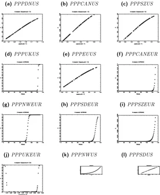
A graphical analysis of the series shown in Figure 1 reveals several
important features: i) all the real exchange rates follow a positively
(negatively) shaped linear broken trend when $ (e) is the numeraire;
ii) the break is located approximately in 2008:04 but continues until
14
first months of 2009, a fact which suggest a regime switching in the
levels; iii) this change in regime is weaker when the e is numeraire
because of the speculative attack during the financial crisis; iv) all
the series show one or more breaks in the middle of the sample,
cor-responding to the selected dummy variables in Table3, two of which
(2003:01 and 2003:03) seem to be consistent with the turbulence
of oil market immediately before and after the Iraqi political crisis
in that months; v) the presence of autocorrelation in rates DN/$ ,
EU/$, DN/e, SD/$, SZ/$ and ARCH-effects is observable in series
in first differences (not reported here). While considering these
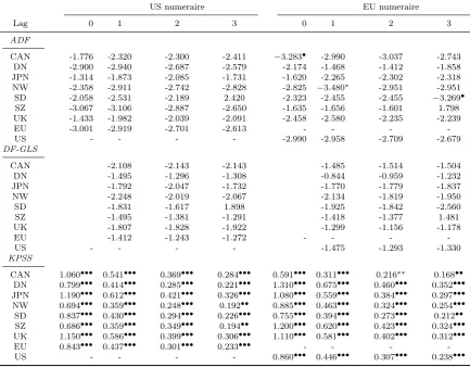
find-ings, it is not a surprise that strong PPP hypothesis does not seem
to hold. Namely we used the Augmented Dikey-Fuller (ADF) test,
the GLS-robust Dikey-Fuller (DF-GLS) (Elliott et al., 1996) for the
null of unit root in the real exchange rates and the KPSS test for
the null of stationarity with a predetermined number of additional
lags (namely, p= 0, . . . ,3) by "Marshallian" approach discussed in
Section3. Table1shows our results: when $ is numeraire we cannot
reject the null of unit root for any country and any lag, while some
exception is observable when e is numeraire but the result is the
same; the only relevant rejection is the case of Norway when testing
for lag 1. The hypothesis of stationarity is almost always rejected
at 1%, regardless to the numeraire, coherently with the above
re-sults. The results for null unit root under GLS estimation confirm
and, possibly, enforce the ADF ones. Clearly, a failure to reject the
null hypothesis of unit root (a rejection of the null of stationarity)
implies an irregularity in the real exchange rate mean reversion and
so a lack of empirical support for strong PPP hypothesis.
5.1
CVAR
For what concerns the CVAR approach for weak PPP hypothesis, the
procedure described in Section 3 is performed in a semi-automatic
way by CATS package (Dennis et al., 2006). Concerning for Step
Ljung-Box LM test for autocorrelation. For simulation of critical values of
Johansen’ Trace test we apply the Johansen (2002) bootstrap
proce-dure with 2,500 draws for each possible rank. For the choice of the
rank, we consider both standard and Bartlett-corrected for small
samples p-values; in a standard scenario, they are really similar.
The plausible restricted models are selected by using the automatic
procedure "CATS Mining", which show all potential cointegrating
relation between covariates and select them as option. Clearly, since
cointegrating relations are simply linear combinations, the number
of candidates is often so high that we have selected them by using the
following criteria: first, p-value of the candidate should be at least
0.20 in order to ensure some stability to the cointegrating relation
which is essential for being economically meaningful, see Juselius
(2006); second, the sign of α and β in (3) should be at least
simi-lar to what theory suggests; finally, their absolute values should not
be extravagant. The presence of I(2)-ness is checked by looking at:
(i) the graphs of the cointegrating relations in their two
specifica-tions: if not strictly similar, this is a sign of I(2) behavior; (ii) the
characteristic roots of the model for a reasonable choice of
cointe-gration rank: if there’s no difference between couples corresponding
the candidate rank and ones immediately after (that is, they are
all near to unit), there’s I(2)-ness; (iii) rank test statistic p-values:
considerable differences between Bartlett and non-Bartlett corrected
p-values. Since the statistical theory of cointegration analysis in an
I(2) scenario is not complete and does not necessarily add
economi-cally meaningful results to the empirical analysis, we stopped when
I(2)-ness was found. Table 3 illustrates our results for PPP when
using $ or e as numeraire. In the majority of cases our optimal lag
choice is 2. However, because of the presence of some outliers, we
will specify the next test forp= 3. Almost all systems do not reject the null of no cointegration, hence, in practice, we stopped to Step 4.
Two exceptions are constituted by Norway and U.K. However, since
other systems, the found relations for these countries are affected by
I(2)-ness15. Moreover, the large number of shift dummies used
cor-responding to an equivalently large number of outliers in residuals
implies that gaussianity assumption of the statistical model could
be seriously suspect to not hold, which is not uncommon in financial
variables.
5.2
Panel methods
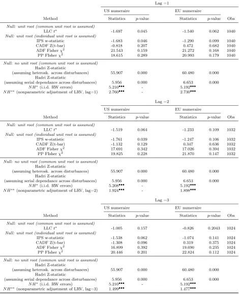
Concerning panel methodology for strong PPP hypothesis, we have
by 8 cross-sections. Since the results country-by country shows that
it’s reasonable to model until p= 3, we test for the first three lags, so that the number of observations varies between 1,024 and 1,040.
The strong PPP hypothesis is investigated by performing the six
tests previously described (see Section 2.3). For MW method we
use both ADF and Phillips-Perron tests. Concerning Hadri test, the
statistic is robust to heteroskedasticity and serial dependance across
disturbances. Table 4 shows that for both numeraires, panel unit
root tests are not able to reject the null hypotheses of unit root with
few exceptions and, coherently with this finding, reject the null of
no unit root. Hence the data do not provide empirical evidence for
strong PPP hypothesis.
The weak PPP hypothesis is investigated by performing the Pedroni
and Westerlund tests on all possible triples of variables. Concerning
Pedroni test, we show only the two most powerful statistics on the
seven proposed by the author, Zρ˜ and ZtρNTˆ . For the same reason,
concerning Westerlund tests, we show only the Pγ statistic. Both of
the tests are based on the null hypothesis of no cointegrating
rela-tion, hence a failure to reject the null hypothesis implies the failure
in finding empirical evidence for weak PPP hypothesis. Notice that
Westerlund test is based on an error correction model, so that,
simi-larly to the CVAR framework, the statistic critical values are biased
15
when allowing for a deterministic kernel to enter in cointegrating
relations. In this case, robust critical values can be computed by
bootstrap methods. Table 5 shows results for each triple, for which
has been provided the statistics, the correspondingz-value, standard
p-value and, for the Westerlund test, bootstrapped p-value and the
automatic selection of lags and leads. The two tests show that spot
rates, domestic and foreign prices are strongly not cointegrated in
two cases on three, regardless to the numeraire, and in the one where
cointegration cannot be rejected the variables are positioned
differ-ently from what theory suggest. This finding leads us to reject the
weak PPP hypotheses, on the contrary of Pedroni (2001).
5.3
Nonlinear models
Concerning the First Puzzle we checked for the presence of
ARCH-effects by performing the McLeod and Li (1983) test before to
im-plement the Granger-Teräsvirta procedure. The results are given in
Table2. We can see that the test fails to reject the null of no
ARCH-effect for almost all the series, but if considering the lag
correspond-ing to the p order of selected model, they became less problematic.
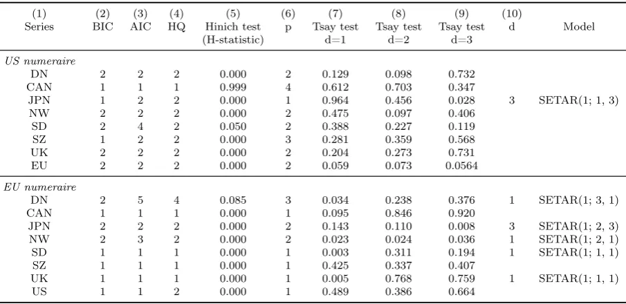
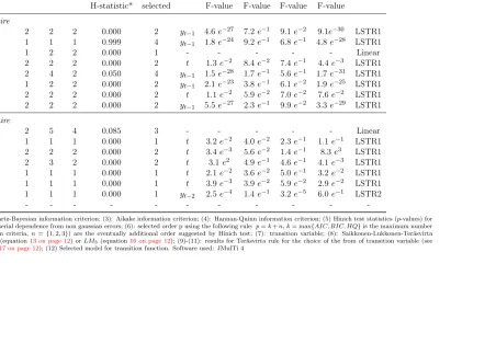
Table8shows the results of the STAR specification procedure above
explained for our dataset. We identified seven LSTR1 models when
$ is numeraire (six when e is numeraire, one of which is LSTR2).
It’s interesting to notice that the errors of the considered series are
not third-order correlated, as suggested by Hinich test: the only case
of correction is CAN/$ (three lag added by procedure described in
Sec. 3). The estimates of selected STAR models are reported in
Table 9.
Figure 2 plots the transition function G(γ, c, st) as function of the
transition variable st. On thirteen estimated nonlinear models, five
(DN/$, CAN/$, SD/$, SZ/$ and e/$) are at the line with linear
models, since their mean reversion is very smooth. The other
mod-els are more clearly nonlinear and, consequently, more interesting
different situations: in the set of models under investigation, the
models NW/$ and SD/$ are the more restricted one, since all lags
of ytN W/$ andySD/$ enter in the restrictionφ=−θ, so the
interpre-tation is very similar to that given in TPS. On the contrary, model
£/e has no restrictions, so there’s no equilibrium around which the
model is a random walk, but more meaningfully a simple
(quasi-exponential) mean reversion; this is the only estimated LSTR2 model
in the dataset. These findings leads to several implications: first, the
methodological choice to not use the restriction for all parameters
jointly and the exponential smooth transition function as a priori
was really critical. Second, the nonlinear asymmetric mean
rever-sion of exchange rates suggests a change in long run, if considering
the TPS’ s implicit observation that goods arbitrage are driving the
market towards it. In this sense, the diagnostic tests in Table10does
not support the idea of a third regime for the estimated model for
any model. Third, and most important, few of the estimated
tran-sition function are puzzling if considering the results form linearity
tests used in Teräsvirta, unless reconsidering the intrinsically
sym-metric (in the sense of Def. 4) structure of the same one in STAR
family. That is, we suspect that such quasi-linear behavior could
be only apparent because data has been forced to be estimated by
using a dynamically symmetric rather than a symmetric statistical
model. In other world, the fact that the econometric literature does
not allow to test for and parametrize an eventual change in the
ve-locity of transition from m1 to ma w.r.t. ma to m2 seems us able
to generate a sort of "neglected dynamic asymmetry" puzzle which
could explain some of the difficulties in fitting a statistically
signifi-cant mean reversion.
Table 9 shows the results for SETAR(k; p, d) specification
proce-dures above explained for our dataset in levels. The Tsay’ s test
allows five currency to be nonlinearly mean-reverting. These results
should not be taken as definitive, since a key role is put on the
SETAR-type nonlinearity but the threshold effect is weak, the nonlinearity
should be interpreted as spurious. This is exactly what happens to
our data. We used all three statistics (11) for testing threshold effect
in both homoskedasticity and heteroskedasticity cases. The p-values
are bootstrapped using 1,000 draws. On six plausible one
thresh-old SETAR models, the threshthresh-old effect hthresh-olds in only one of them,
namely in the real exchange rate £/eas shown in Table 7.
More-over, this is a limit-case, since only thesupST-statistic is in rejection
region, when the test is robust to heteroskedasticity. These are the
resulting estimates where the values in brackets are robust standard
errors:
yt£/e =−0.022 + 0.849·yt£−/e1 if yt£−/e1 ≤0.341, σˆ2 = 0.0007
(0.013) (0.055)
yt£/e = 0.006 + 0.984·y
£/e
t−1 if y
£/e
t−1 >0.341, σˆ2 = 0.0002
(0.011) (0.026)
(20)
An interesting feature is that the estimated SETAR model (as all
plausible threshold models, too) are not so sensitive to
heteroskedas-ticity, and the above model is the only exception. That is, the
rel-evant ARCH-effects showed in Table 2 does not involve any
rele-vant difference in (bootstrapped) p-values when performing an
het-eroskedasticity robust test for threshold effect respect on the
non-robust one.
Concerning the Second Puzzle, the previously introduced "neglected
dynamic asymmetry puzzle" leads us to not follow TPS pedantically
in using the GRT method for GIRF analysis in order to study the
shocks persistence of real exchange rates and to use TIRF for the
five models previously mentioned. Nevertheless, neither in the other
series we agree in performing the GRT method, since our modeling
strategy and the resulting models was different from TPS: their
so-lution to PPP puzzle was based on ESTAR model, which has been
shown in Section 2.4 to be a very peculiar case of the more general
is an LSTR2, since c1 6=c2; this means that the transition function
is not perfectly symmetric (neither in the common meaning of the
term, although it can be seen as an approximation), hence the
eco-nomic interpretation of the resulting GIRF could be misleading16.
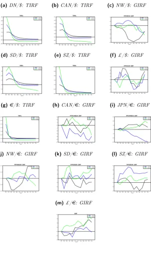
Figure 3 plots the TIRF/GIRF of the real exchange rate series for
shocks of magnitude {1, 2, 3} and an horizon of 12 month. It’s easy
to notice the different behavior of the two groups: in TIRFs, when
the shock is larger (shock=3, green line) the TIRF does converge
faster to 0 and tends immediately to go slightly below such
thresh-old; more in general, a common feature of all the TIRFs is that small
shocks tend to disappear slower than big shocks (6-8 months against
2-4) month. This confirms in some way the TPS result, showing the
nonlinearity of the real exchange rate adjustment toward theoretical
PPP equilibrium. On the other hand, when considering the GIRFs,
the shocks are more problematic, since they does not seem to have
a clear path. It’s interesting to note that TPS concerns for a larger
scaled dataset17 so that our result can be seen, nevertheless all the
mentioned empirical problems, as a reasonable approximation to it.
6
Conclusions
In this article we studied the empirical support for the PPP
the-ory after 1998 by using different methodologies in both linear and
nonlinear scenario in order to compare and update the available
em-pirical literature.
The general result is ambivalent: the analysis of a dataset of 16
real exchange rates does not support the PPP hypothesis when a
linear scenario is used. In particular, the CVAR analysis show the
16
Moreover, the GRT method for GIRF is based on several strong assump-tion: parametric distribution; the mean as statistic measure of baseline forecasts,
"[. . . ] which under stationarity is the unconditional mean" (Koopet al.(1996,
pag.130)); the GIRF is zero if the initial shock is zero. We note that the second assumption is the most problematic one because when shocks have asymmet-ric effect,"[. . . ] then averaging across phases of the business cycle will tend to
weaken or hide the evidence of asymmetry"(Ibidem).
17
two cases in which weak PPP holds are found to be strongly I(2).
Panel methods for unit root and cointegration confirm the rejection
of the theory, although the BMO’s critique suggests to take such
re-sults very carefully. Things seem different in the nonlinear scenario:
13 rates on 16 are nonlinearly mean reverting, where the change in
regime is located in correspondence of the crisis. This implies that
the financial crisis in 2008 has been a source of nonlinear
behav-ior which allowed to explain the movements for some rates better
than using a linear framework. In particular, two findings are
puz-zling: first, the qualitative analysis of the nonlinear part of several
STAR models shows a quasi-linear transition function, a fact that
leads us to suspect a sort of neglected dynamic asymmetry in
tran-sition functions due to a gap in the econometric methodology used.
Second, data are not able to support the choice of an ESTAR-type
of nonlinearity in favor of an LSTAR-type; that is, contrarily to
TPS, the speed of adjustment of exchange rates varies according to
the over(under)valuation of the numeraire. We conclude that the
solution of the two PPP puzzles needs a methodological approach
slightly different form the TPS one when considering a nonlinear
scenario. In particular, the problem of capturing the effect of the
dynamically asymmetry in model parameters is still today unsolved
by the econometric literature. Hence standard nonlinear models can
be reasonably used only when strongly nonlinear transition functions
are estimated. Our modified General-to-Specific modelling strategy
seems being an help but only as a very preliminary step. However, for
what concerns the Second Puzzle, TIRFs for estimated real exchange
rates for an horizon of one year confirm the nonlinear adjustment of
the real exchange rates towards their theoretical PPP value and, in
an approximate way, the TPS result. This is consistent with the
eco-nomic intuition underlying the use of LSTAR as transition function:
in period of crisis shocks in real exchange rates tends to no return
to their previous level.
the multivariate scenario could be the natural extension of this work,
but the problem of neglected asymmetry before mentioned could be
exacerbated. For this reason we think that relaxing the assumption
of symmetry in transition functions could be a preferable strategy.
This would require a re-examination of the whole structure of STR
family. We remind this extension to further works.
References
Banerjee, A., Marcellino, M. and Osbat, C. (2005). Testing
for PPP: Should we use panel methods? Empirical Economics,
30, 77–91, DOI: 10.1007/s00181-004-0222-8.
Coleman, A.(1995). Arbitrage, Storage and the Law of One Price:
New Theory for the Time Series Analysis of an Old Problem. Dis-cussion Paper. Department of Economics. Princeton University.
Dennis, J.,Hansen, H., Johansen, S.andJuselius, K.(2006).
CATS in RATS. Cointegration Analysis of Time Series, Version 2. Estima: Evanston.
Eitrheim, O.andTeräsvirta, T.(1996). Testing the adequacy of
smooth transition autoregressive models.Journal of Econometrics,
74, 59–75, DOI: 10.1016/0304-4076(95)01751-8.
Elliott, G., Rothemberg, T. and Stock, J. (1996). Efficient
Tests for an Autoregressive Unit Root. Econometrica, 64, 813–
836.
Gadea, M. and Mayoral, L.(2009). Aggregation is Not the
So-lution: The PPP Strikes Back.Journal of Applied Econometrics,
24, 875–894, DOI: 10.1002/jae.1078.
Gallant, A., Rossi, P.and Tauchen, G. (1993). Nonlinear
Dy-namic Structures.Econometrica, 61, 871–907.
Granger, C. and Teräsvirta, T. (1993). Modelling Nonlinear
Economic Relationships. Oxford: Oxford University Press.
Hadri, K. (2000). Testing for stationarity in heterogeneous panel
data. Econometrics Journal, 3, 148–161, DOI:
10.1111/1368-423X.00043.
Hansen, B. (1996). Inference when a nuisance parameter is not
Hinich, M. (1996). Testing for dependence in the input to a linear time series model.Journal of Nonparametric Statistic,6, 205–221,
DOI: 10.1080/10485259608832672.
Im, K., Pesaran, M. and Shin, Y. (2003). Testing for unit roots
in heterogeneous panels. Journal of Econometrics, 115, 53–74.
Imbs, J.,Muntaz, H.,Ravn, M.andRey, H.(2005). PPP Strikes
Back: Aggregation and Real Exchange Rate.Quarterly Journal of
Economics, 120 (1), 1–43.
Johansen, S. (1991). Estimation and Hypothesis Testing of
Coin-tegrating Vectors in Gaussian Vectors Autoregressive Models.
Econometrica., 59, 1551–1580.
— (2002). A small sample correction for tests of hypotheses on the
cointegrated vectors.Journal of Econometrics, 111, 195–221.
—, Juselius, K., Frydman, R. and Goldberg, M. (2010).
Testing hypotheses in an I(2) model with piecewise linear trends. An analysis of the persistent long swings in the
Dmk/$ rate. Journal of Econometrics, 158, 117–129, DOI:
10.1016/j.jeconom.2010.03.018.
Juselius, K. (2006). The Cointegrated VAR Model: Methodology
and Applications. Oxford: Oxford University Press.
— (2009). The Long Swings Puzzle: What the Data Tell When
Allowed to Speak Freely. In K. Patterson and T. Mills (eds.),
The Palgrave Handbook of Empirical Econometrics, Macmillan, pp. 367–384.
Koop, G., Pesaran, M. and Potter, S. (1996). Impulse
Re-sponse Analysis in Nonlinear Multivariate Models. Journal of
Econometrics,74, 119–147, DOI: 10.1016/0304-4076(95)01753-4.
Kwiatkowski, D., Phillips, P., Shmidt, P. and Shin, Y.
(1992). Testing the null hypothesis of stationarity against the al-ternative of a unit root: How sure are we that economic time
series have a unit root? Journal of Econometrics, 54, 159–178,
DOI: 10.1016/0304-4076(92)90104-Y.
Levin, A.,Lin, C.andChu, C.(2002). Unit root test in panel data:
Asymptotic and finite sample properties.Journal of Econometrics,
87, 207–237, DOI: 10.1016/S0304-4076(01)00098-7.
Luukkonen, R., Saikkonen, P. and Teräsvirta, T. (1988).
Testing linearity against smooth transition autoregressive models.
Maddala, G. and Wu, S. (1999). A comparative study of unit
root tests with panel data and a new simple test. Oxford Bulletin
of Economics and Statistics, 61, 631–652, DOI:
10.1111/1468-0084.0610s1631.
McLeod, A. and Li, W. (1983). Diagnostic checking ARMA
time series models using squared-residual autocorrelations.
Jour-nal of Time Series AJour-nalysis, 4, 269–273, DOI:
10.1111/j.1467-9892.1983.tb00373.x.
Nyblom, J. and Harvey, A. (2000). Tests of Common Stochastic
Trends. Econometric Theory, 16, 176–199.
Pedroni, P. (2001). Purchasing power parity tests in cointegrated
panels. The Review of Economics and Statistics, 83, 727–731,
doi:10.1162/003465301753237803.
— (2004). Panel cointegration: asymptotic and finite sample
properties of pooled time series tests with an application to
the PPP hypothesis. Econometric Theory, 20, 597–625, DOI:
10.1017/S0266466604203073.
Pesaran, M. (2007). A Simple Panel Unit Root Test for
Cross-Section Dependance. Journal of Applied Econometrics, 22, 265–
312, DOI: 10.1002/jae.951.
Rogoff, K. (1996). The Purchasing Power Parity Puzzle. Journal
of Economic Literature,34, 647–668.
Sarno, L. and Taylor, M. (2001). Purchasing Power Parity and
the Real Exchange Rates. CEPR Discussion Papers 2913.
Taylor, M., Peel, D. and Sarno, L. (2001). Nonlinear Mean
Reversion in Real Exchange Rates: Towards a Solution to the
Purchasing Power Parity Puzzles.International Economic Review,
pp. 1015–1042, DOI: 10.1111/1468-2354.0014.
Teräsvirta, T.(1994). Specification, estimation and evaluation of
smooth transition autoregressive models.Journal of the American
Statistical Association,89, 208–218.
— (2006). Forecasting Economic Variables with Nonlinear Models.
In G. Elliott, C. Granger and A. Timmermann (eds.), Handbook
of Economic Forecasting, vol. 1, Elsevier BV., pp. 414–457.
Tsay, R.(1989). Testing and modeling threshold autoregressive
pro-cesses. Journal of the American Statistical Association, 84, 231–
240.
Westerlund, J. (2007). Testing for Error Correction in Panel
Data. Oxford Bulletin of Economics and Statistics, 69, 709–748,
A
Appendix
A.1
Data
Our original dataset is constituted of monthly series of spot rates (cur-rency basis United States Dollar and Euro) and consumers’ price indices. Sample: 1999:01-2009:12 (132 observation). Spot rate series with basis USD source: FED of St. Louis. Series names:
Canada: EXCAUS, Board of Governors of Federal Reserve System; Denmark: EXDNUS, Board of Governors of Federal Reserve System; Japan: EXJPUS, Board of Governors of Federal Reserve System; Norway: EXNOUS, Board of Governors of Federal Reserve System; Sweden: EXSDUS, Board of Governors of Federal Reserve System; Switzerland: EXSZUS,Board of Governors of Federal Reserve System; U.K.: United Kingdom, Exchange Rates, OECD;
EU: EU-12-Extra EU, Exchange Rates, OECD.
Spot rate time series with basis EUR source: European Central Bank. Dataset name: Exchange Rates; frequency: monthly; currency denomi-nator: Euro; exchange rate type: spot; series variation - EXR context: average or standardized measure for given frequency. Series names: Canadian dollar: EXR.M.CAD.EUR.SP00.A;
Danish krone: EXR.M.DKK.EUR.SP00.A; Japanese yen: EXR.M.JPY.EUR.SP00.A; Norwegian krone: EXR.M.NOK.EUR.SP00.A; Swedish krona: EXR.M.SEK.EUR.SP00.A; Swiss franc: EXR.M.CHF.EUR.SP00.A;
U.K. pound sterling: EXR.M.GBP.EUR.SP00.A; U.S. dollar: EXR.M.USD.EUR.SP00.A.
CPI series source: OECD. Series names:
Canada: CAN CPI - All items - Index publication base - units: 2005=100; Denmark: DNK CPI - All items - Index publication base - units: 2005=100; Japan: JPN CPI - All items Tokyo - Index publication base - units: 2005=100;
Norway: NOR CPI - All items - Index publication base - units: 2005=100; Sweden: SWE CPI - All items net - Index publication base - units: 2005=100;
Switzerland: CHE CPI - All items - Index publication base - units: 2005=100;
U.K.: GBR CPI - All items - Index publication base - units: 2005=100; U.S: USA CPI - All items SA - Index publication base - units: 2005=100; E.U.: EMU CPI HICP - All items - Index publication base - units: 2005=100.
A.2
Tables and Graphs
Table 1: Univariate Tests on Real Exchange Rates
US numeraire EU numeraire
Lag 0 1 2 3 0 1 2 3
ADF
CAN -1.776 -2.320 -2.300 -2.411 −3.283• -2.990 -3.037 -2.743
DN -2.900 -2.940 -2.687 -2.579 -2.174 -1.468 -1.412 -1.858
JPN -1.314 -1.873 -2.085 -1.731 -1.620 -2.265 -2.302 -2.318
NW -2.358 -2.911 -2.742 -2.828 -2.825 −3.480∗ -2.951 -2.951
SD -2.058 -2.531 -2.189 2.420 -2.323 -2.455 -2.455 −3.269•
SZ -3.067 -3.106 -2.887 -2.650 -1.635 -1.656 -1.601 1.798
UK -1.433 -1.982 -2.039 -2.091 -2.458 -2.580 -2.235 -2.239
EU -3.001 -2.919 -2.701 -2.613 - - -
-US - - - - -2.990 -2.958 -2.709 -2.679
DF-GLS
CAN -2.108 -2.143 -2.143 -1.485 -1.514 -1.504
DN -1.495 -1.296 -1.308 -0.844 -0.959 -1.232
JPN -1.792 -2.047 -1.732 -1.770 -1.779 -1.837
NW -2.248 -2.019 -2.067 -2.134 -1.819 -1.950
SD -1.831 -1.617 1.898 -1.925 -1.842 -2.560
SZ -1.495 -1.381 -1.291 -1.418 -1.377 1.481
UK -1.807 -1.828 -1.922 -1.299 -1.156 -1.178
EU -1.412 -1.243 -1.272 - - -
-US - - - - -1.475 -1.293 -1.330
KPSS
CAN 1.060••• 0.541••• 0.369••• 0.284••• 0.591••• 0.311••• 0.216∗∗ 0.168••
DN 0.799••• 0.414••• 0.285••• 0.221••• 1.310••• 0.675••• 0.460••• 0.352•••
JPN 1.190••• 0.612••• 0.421••• 0.326••• 1.080••• 0.559••• 0.384••• 0.297•••
NW 0.694••• 0.359••• 0.248••• 0.192•• 0.885••• 0.463••• 0.324••• 0.254•••
SD 0.837••• 0.430••• 0.294••• 0.226••• 0.755••• 0.394••• 0.273••• 0.212••
SZ 0.686••• 0.359••• 0.349••• 0.194•• 1.200••• 0.620••• 0.423••• 0.324•••
UK 1.150••• 0.586••• 0.399••• 0.306••• 1.110••• 0.581••• 0.402••• 0.312•••
EU 0.843••• 0.437••• 0.301••• 0.233••• - - -
-US - - - - 0.860••• 0.446••• 0.307••• 0.238•••
•Rejection at 10% of the null hypothesis; ••rejection at 5% of the null hypothesis; • • •
[image:33.595.100.453.613.737.2]rejection at 1% of the null hypothesis. Software used: RATS 7.2
Table 2: McLeod-Li test for no ARCH-effects in∆PPP (p-value)
US numeraire EU numeraire
Lag 1 2 3 4 1 2 3 4
DN 0.442 0.013 0.034 0.049 0.753 0.839 0.894 0.502
CAN 0.867 0.732 0.847 0.937 0.807 0.969 0.592 0.489
JPN 0.152 0.082 0.171 0.285 0.000 0.000 0.000 0.000
NW 0.000 0.000 0.001 0.002 0.017 0.000 0.000 0.000
SD 0.009 0.032 0.048 0.092 0.097 0.016 0.013 0.014
SZ 0.115 0.247 0.320 0.471 0.380 0.427 0.023 0.047
UK 0.000 0.000 0.000 0.000 0.011 0.015 0.022 0.039
US - - - - 0.048 0.012 0.031 0.056
EU 0.175 0.004 0.010 0.012 - - -