http://dx.doi.org/10.4236/ajor.2013.36048
A Computational Comparison of Basis Updating Schemes
for the Simplex Algorithm on a CPU-GPU System
Nikolaos Ploskas*, Nikolaos Samaras
Department of Applied Informatics, School of Information Sciences, University of Macedonia, Thessaloniki, Greece Email: *[email protected]
Received August 19, 2013; revised September 19, 2013; accepted September 29,2013
Copyright © 2013 Nikolaos Ploskas, Nikolaos Samaras. This is an open access article distributed under the Creative Commons At-tribution License, which permits unrestricted use, disAt-tribution, and reproduction in any medium, provided the original work is prop-erly cited.
ABSTRACT
The computation of the basis inverse is the most time-consuming step in simplex type algorithms. This inverse does not have to be computed from scratch at any iteration, but updating schemes can be applied to accelerate this calculation. In this paper, we perform a computational comparison in which the basis inverse is computed with five different updating schemes. Then, we propose a parallel implementation of two updating schemes on a CPU-GPU System using MAT- LAB and CUDA environment. Finally, a computational study on randomly generated full dense linear programs is pre- sented to establish the practical value of GPU-based implementation.
Keywords: Simplex Algorithm; Basis Inverse; Graphics Processing Unit; MATLAB; Compute Unified Device
Architecture
1. Introduction
Linear Programming (LP) is the process of minimizing or maximizing a linear objective function to a number of linear equality and inequality constraints. Simplex algo- rithm is the most widely used method for solving Linear Programming problems (LPs). Consider the following linear programming problem in the standard form shown in Equation (1):
min subject to 0
T
c x
Ax b
x
(1)
where ARm n ,
c x,
Rn, bRm, andT denotes
transposition. We assume that A has full rank, rank(A) = m, m < n. Consequently, the linear system Ax = b is con-
sistent. The simplex algorithm searches for an optimal solution by moving from one feasible solution to another, along the edges of the feasible set. The dual problem associated with the linear problem in Equation (1) is shown in Equation (2):
min subject to 0
T T
b w
A w s c
s
(2)
where m
wR and n
sR .
The past twenty years have been a time of remarkable developments in optimization solvers. Real life LPs tend to be large in size. A growing number of problems de- mand parallel computing capabilities. The explosion in computational power (CPUs and GPUs) has made it pos- sible to solve large and difficult LPs in a short amount of time. As in the solution of any large scale mathematical system, the computational time for large LPs is a major concern. The basis inverse dictates the total computa- tional effort of an iteration of simplex type algorithms. This inverse does not have to be computed from scratch at any iteration, but can be updated through a number of updating schemes. All efficient versions of the simplex algorithm work with some factorization of the basis ma- trix B or its inverse B−1.
Dantzig and Orchard-Hays [1] have proposed the Product Form of the Inverse (PFI), which maintains the basis inverse using a set of eta vectors. Benhamadou [2] proposed a Modification of the Product Form of the In- verse (MPFI). The key idea is that the current basis in- verse
AB 1 can be computed from the previous in-verse
AB 1
using a simple outer product of two vec- tors and one matrix addition.
LU decomposition produces generally sparser factori- zations than PFI [3]. The LU factorization for the basis inverse has been proposed by Markowitz [4]. Markowitz used LU decomposition to fully invert a matrix, but used the PFI scheme to update the basis inverse during sim- plex iterations. Bartels and Golub [5] have later proposed a scheme to update a sparse factorization, which was more stable than using PFI. Their computational experi- ments, however, proved that it was more computationally expensive. Forrest and Tomlin [6] created a variant of the Bartels-Golub method by sacrificing some stability char- acteristics causing the algorithm to have a smaller growth rate in the number of non-zero elements relative to the PFI scheme. Reid [7] proposed two variants of the Bar- tels-Golub updating scheme that aim to balance the spar- sity and the numerical stability of the factorization. A variant of the Forrest-Tomlin update was proposed by Suhl and Suhl [8]. Other important updating techniques can be found in Saunders [9] and Goldfarb [10]. A full description of most of these updating methods can be found in Nazareth [11] and Chvátal [12].
There have been many reviews and variants of these methods individually, but only a few comparisons be- tween them that are either obsolete or don’t compare all these updating schemes. McCoy and Tomlin [13] report the results of some experiments on measuring the accu- racy of the PFI scheme, Bartels-Golub method and Forrest- Tomlin scheme. Lim et al. [14] provide a comparative
study between Bartels-Golub method, Forrest-Tomlin method and Reid method. Badr et al. [15] perform a
computational evaluation of PFI and MPFI updating schemes. Ploskas et al. [16] compare PFI and MPFI up-
dating schemes both on their serial and their parallel im- plementation.
Originally, GPUs used to accelerate graphics rendering. GPUs have gained recently a lot of popularity and High Performance Computing applications have already start- ed to use them. The computational capabilities of GPUs exceed the one of CPUs. GPU is utilized for data parallel and computationally intensive portions of an algorithm. NVIDIA introduced Compute Unified Device Architec- ture (CUDA) in late 2006. CUDA enables users to exe- cute codes on their GPUs and it is based on a SIMT pro- gramming model. Any performance improvements in the parallelization of the revised simplex algorithm would be of great interest. Using GPU computing for solving large- scale LPs is a great challenge due to the capabilities of GPU architectures.
Some related works have been proposed on the GPU parallelization for LPs. O’Leary and Jung [17] proposed a CPU-GPU implementation of the Interior Point Method for dense LPs. Their computational results on Netlib Set [18] showed that some speedup can be gained for large dense problems. Spampinato and Elster [19] presented a
GPU-based implementation of the Revised Simplex Al- gorithm on GPU with NVIDIA CUBLAS [20] and NVIDIA LAPACK libraries [21]. Their implementation showed a maximum speedup of 2.5 on randomly gener- ated LPs of at most 2000 variables and 2000 constraints. Bieling et al. [22] also proposed a parallel implementa-
tion of the Revised Simplex Algorithm on GPU. They compared their GPU-based implementation with GLPK solver and found a maximum speedup of 18 in single precision. Lalami et al. [23] proposed a parallel imple-
mentation of the standard Simplex on a CPU-GPU sys- tems. Their computational results on randomly generated dense problems of at most 4000 variables and 4000 con- straints showed a maximum speedup of 12.5. Meyer et al.
[24] proposed a mono and a multi-GPU implementation of the standard Simplex algorithm and compared their implementation with the CLP solver. Their implementa- tion outperformed CLP solver on large sparse LPs. Li et al. [25] presented a GPU-based parallel algorithm, based
on Gaussian elimination, for large scale LPs that outper- form the CPU-based algorithm.
This paper presents a computational study in which the basis inverse is computed with five different updating schemes: 1) Gaussian elimination; 2) the built-in func- tion inv of MATLAB; 3) LU decomposition; 4) product
form of the inverse; and 5) a modification of the prod- uct form of the inverse; and incorporates them with the revised simplex algorithm. Then, we propose a parallel implementation of PFI and MPFI schemes, which were the fastest among the five updating methods, on a CPU-GPU System, which is based on MATLAB and CUDA.
The structure of the paper is as follows. In Section 2, a brief description of the revised simplex algorithm is pre- sented. In Section 3, five methods that have been widely used for basis inversion are presented and analyzed. Sec- tion 4 presents the computational comparison of the se- rial implementations of the updating schemes. Computa- tional tests were carried out on randomly generated LPs of at most 5000 variables and 5000 constraints. Section 5 presents the GPU-based implementations of two updat- ing schemes. In Section 6, a computational study of the GPU-based implementations is performed. Finally, the conclusions of this paper are outlined in Section 7.
2. Revised Simplex Method
Using a partition (B, N) Equation (1) can be written as
shown in Equation (3): min subject to
, 0
T T
B B N N
B B N N
B N
c x c x
A x A x b
x x
(3)
matrix of A, called basic matrix or basis. The columns of A belonging to subset B are called basic and those be-
longing to N are called non-basic. The solution of the
linear problem 1 , 0
B B N
x A b x is called a basic solu- tion. A solution x
xB,xN
is feasible iff x0; oth-erwise the solution is infeasible. The solution of the lin- ear problem in Equation (2) is computed by the relation
T
s c A w , where w
cB T AB1 are the simplexmultipliers and s are the dual slack variables. The basis AB is dual feasible iff s0.
In each iteration, simplex algorithm interchanges a col- umn of matrix AB with a column of matrix AN and con-
structs a new basis AB. Any iteration of simplex type
algorithms is relatively expensive. The total work of an iteration of simplex type algorithms is dictated by the computation of the basis inverse. This inverse, however, does not have to be computed from scratch during each iteration of the simplex algorithm. Simplex type algo- rithms maintain a factorization of basis and update this factorization in each iteration. There are several schemes for updating basis inverse. In Section 3, we present eight well-known methods for the basis inverse. A formal de- scription of the revised simplex algorithm [26] is pre- sented in Table 1.
3. Basis Inversion Updating Schemes
3.1. Gaussian Elimination
[image:3.595.357.492.608.731.2]Gaussian elimination is a method for solving systems of linear equations, which can be used to compute the in- verse of a matrix. Gaussian elimination performs the
Table 1. Revised simplex algorithm.
Step 0. (Initialization).
Start with a feasible partition (B, N). Compute AB 1
and vec-tors xB, w and sN.
Step 1. (Test of optimality).
if sN0 then
STOP. The linear problem is optimal. else
Choose the index l of the entering variable using a pivoting rule.
Variable xl enters the basis.
Step 2. (Minimum ratio test).
Compute the pivot column hl AB 1Al.
if hl0 then
STOP. The linear problem is unbounded. else
Choose the leaving variable xk = xB[r] using the Equation (4):
min : 0
B r B i
il B r il il x x x h h h
(4)
Step 3. (Pivoting).
Swap indices k and l. Update the new basis inverse
AB 1, usingan updating scheme. Go to Step 1.
following two steps: 1) Forward Elimination: reduces the given matrix to a triangular or echelon form and 2) Back Substitution: finds the solution of the given system. Gaussian elimination with partial pivoting requires O(n3)
time complexity.
Gaussian elimination has been implemented on MAT- LAB using the mldivide operator. In order to find the
new basis inverse using Gaussian elimination, one can use the Equation (5):
1\
B B
A A I (5)
3.2. Built-In Function Inv of MATLAB
The basis inverse can be computed using the built-in function of MATLAB called inv, which uses LAPACK
routines to compute the basis inverse. Due to the fact that this function is already compiled and optimized for MATLAB, its execution time is smaller compared with the other relevant methods that compute the explicit basis inverse; time-complexity, though, remains O(n3).
3.3. LU Decomposition
LU decomposition method factorizes a matrix as the product of an upper U and a lower L triangular factors, which can be used to compute the inverse of a matrix. In order to compute the U and L factors, the built-in func- tion of MATLAB called lu has been used. LU decompo- sition can be computed in time O(n3).
3.4. MPFI
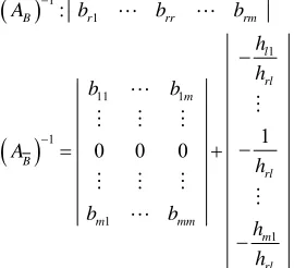
MPFI updating scheme has been presented by Ben- hamadou [3]. The main idea of this method is that the current basis inverse
AB 1 can be computed from the previous inverse
AB 1
using a simple outer product of two vectors and one matrix addition, as shown in the Equation (6):
1 1
1.
. B
B B r r
A A v A (6) The updating scheme of the inverse is shown in Equa- tion (7).
1 1 1 11 1 1 1 1 : 10 0 0
B r rr rm
l rl m B rl m mm m rl
A b b b
The outer product of Equation (7) requires m2 multi-
plications and the addition of two matrices requires m2
additions. Hence, the complexity is
2 m .
3.5. PFI
The PFI scheme, in order to update the new basis
AB 1,uses information only about the entering and leaving variables along with the current basis
AB 1
. The new basis inverse can be updated at any iteration using the Equation (8).
1
1 1( )1B B
B
A A E E A (8)
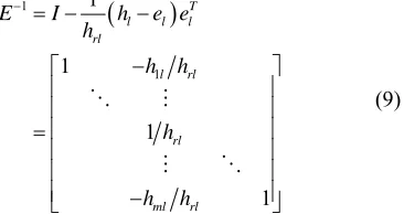
where E−1 is the inverse of the eta-matrix and can be
computed by the Equation (9):
1
1
1
1
1
1 T
l l l
rl
l rl
rl
ml rl
E I h e e
h
h h
h
h h
(9)
If the current basis inverse is computed using regular multiplication, then the complexity of the PFI is
3m
.
4. Computational Results of Serial
Implementations
Computational studies have been widely used, in order to examine the practical efficiency of an algorithm or even compare algorithms. The computational comparison of the aforementioned five updating schemes has been per- formed on a quad-processor Intel Core i7 3.4 GHz with 32 Gbyte of main memory running under Microsoft Windows 7 64-bit. The algorithms have been imple- mented using MATLAB Professional R2012a. MAT- LAB (MATrix LABoratory) is a powerful programming environment and is especially designed for matrix com- putations in general. All times in the following tables are measured in seconds.
[image:4.595.106.289.273.370.2]The test set used in the computational study was ran- domly generated. Problem instances have the same num- ber of constraints and variables. The largest problem tested has 5000 constraints and 5000 variables. All in- stances are dense. For each instance, we averaged times over 10 runs. A time limit of 20 hours was set that ex- plains why there are no measurements for some updating methods on large instances. It should be noted that in MATLAB R2012a multithreading is enabled by default thus our implementations are automatically parallelized and executed using the available multicore CPU.
Table 2 presents the results from the execution of the
above mentioned updating schemes. We have also in- cluded the execution time from MATLAB’s linprog
built-in function, a function for solving linear program- ming problems. MATLAB’s linprog function includes
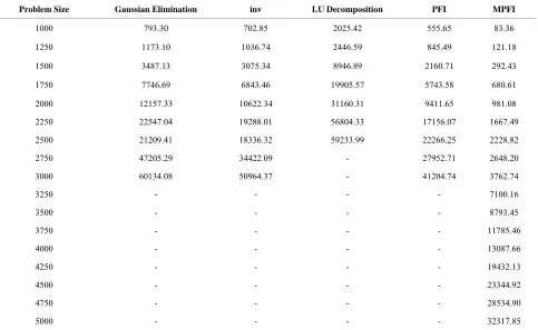
two algorithms for large-scale and medium-scale opti- mization. The large-scale algorithm is based on Interior Point Solver [27], a primal-dual interior-point algorithm. LIPSOL used a Cholesky-infinity factorization that caus- es overhead during the factorization of dense matrices and as a result it cannot solve problems with more than 1500 variables and constraints. Due to this restriction, we have used in our comparison the medium-scale algorithm, which is a variation of the simplex method. Table 3 in-
cludes the execution time for the basis inverse of each updating scheme, while Table 2 presents the total exe-
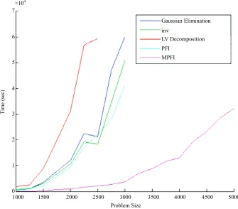
cution time. The execution time of the basis inverse and the whole algorithm for each updating scheme is also graphically illustrated in Figures 1 and 2, respec-
tively.
The MPFI updating scheme has the best performance. On the other hand, LU updating method has the worst performance. Another significant issue is the perform- ance of Gaussian elimination, PFI, function inv and lin- prog of MATLAB which are close to each other and the
results are not quite satisfactory.
5. Parallel Implementation of PFI and MPFI
Updating Schemes on a CPU-GPU System
PFI and MPFI were the fastest updating schemes. In this section, we present the GPU-based implementations of these updating methods taking advantage of the power that modern GPUs offer. The parallel implementations of these updating methods are implemented on MATLAB and CUDA. The updating methods are built using both native MATLAB code and CUDA MEX files.Both methods take as input the previous basis inverse
1B
A , the pivot column hl, the index of the leaving
variable (k) and the number of the constraints (m).
5.1. GPU-Based MPFI
Let us assume that we have t gpu cores. Table 4 shows
the steps that we used to compute the new basis inverse
1B
A with the MPFI scheme on the GPU.
5.2. GPU-Based PFI
Table 5 shows the steps that we used to compute the new
basis inverse
AB 1 with the PFI scheme on the GPU.6. Computational Results of Parallel
Implementations
Table 2. Total time (secs).
Problem Size Gaussian Elimination inv LU Decomposition PFI MPFI linprog
1000 871.81 774.15 2314.62 631.22 155.51 171.68
1250 1269.92 1134.50 2820.17 940.03 216.97 3453.09
1500 3746.93 3330.55 10351.52 2384.46 509.71 7097.17
1750 8245.07 7347.78 23153.03 6255.89 1161.56 11682.54
2000 12875.85 11340.48 36338.81 10140.09 1670.73 19267.61
2250 23709.13 20453.34 66437.50 18345.68 2798.21 36614.81
2500 34249.22 22975.68 63775.88 23828.22 3730.49 44998.08
2750 49312.02 36202.77 - 29762.26 4384.83 -
3000 62646.43 53472.82 - 43740.40 6242.79 -
3250 - - - - 14200.80 -
3500 - - - - 20147.04 -
3750 - - - - 28776.84 -
4000 - - - - 34235.18 -
4,250 - - - - 42196.15 -
4500 - - - - 51210.67 -
4750 - - - - 62919.07 -
5000 - - - - 70058.59 -
Table 3. Basis inverse time (secs).
Problem Size Gaussian Elimination inv LU Decomposition PFI MPFI
1000 793.30 702.85 2025.42 555.65 83.36
1250 1173.10 1036.74 2446.59 845.49 121.18
1500 3487.13 3075.34 8946.89 2160.71 292.43
1750 7746.69 6843.46 19905.57 5743.58 680.61
2000 12157.33 10622.34 31160.31 9411.65 981.08
2250 22547.04 19288.01 56804.33 17156.07 1667.49
2500 21209.41 18336.32 59233.99 22266.25 2228.82
2750 47205.29 34422.09 - 27952.71 2648.20
3000 60134.08 50964.37 - 41204.74 3762.74
3250 - - - - 7100.16
3500 - - - - 8793.45
3750 - - - - 11785.46
4000 - - - - 13087.66
4250 - - - - 19432.13
4500 - - - - 23344.92
4750 - - - - 28534.90
[image:5.595.57.540.439.736.2]1000 1500 2000 2500 3000 3500 4000 4500 5000 Problem Size
0 1
T
im
e (se
c)
Gaussian Elimination
2 3 4 5 6 7
×104
inv
LV Decomposition PFI
[image:6.595.125.460.86.380.2]MPFI
Figure 1. Basis inverse time comparison.
1000 1500 2000 2500 3000 3500 4000 4500 5000
Problem Size 0
1
T
ime
(s
ec
)
Gaussian Elimination
2 3 4 5 6 7 8
×104
inv
LV Decomposition PFI
[image:6.595.127.463.393.710.2]MPFI linprog
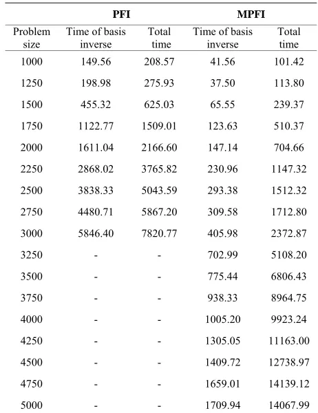
order to test the performance of the GPU-based imple- mentations. The computational comparison of the paral- lel implementations has been also performed on a quad- processor Intel Core i7 3.4 GHz with 32 Gbyte of main memory running under Microsoft Windows 7 64-bit and NVIDIA Quadro 6000 with 6 Gbyte of memory and 448 CUDA cores. The mex files have been implemented us- ing CUDA 4.2 and Microsoft Visual Studio 2012. Table 6 presents the results from the execution of the GPU-
based implementations of PFI and MPFI updating schemes. For each implementation, the table shows the CPU time for the basis inverse and the total time.
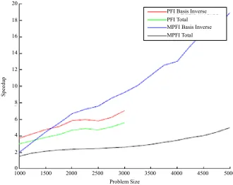
Table 7 presents the speedup obtained by the GPU-
based implementations regarding the CPU time for the basis inverse and the total time. We now plot the ratios taken from Table 7 in Figure 3. The total time is in loga-
rithmic scale.
From the results, we observe: 1) the MPFI scheme is much faster than PFI both in serial and in GPU-based implementation, 2) using PFI scheme, the speedup gained from the GPU implementation is around 7 for the time of basis inverse and 5.5 for total time when the
Table 4. GPU-based MPFI.
Step 0.
Compute the column vector:
T
1l ml
rl rl rl
h 1 h
v
h h h
Each core computes in parallel m/t elements of v. The pivot
ele-ment is shared between all t cores.
Step 1.
Compute the outer product 1
.
B r
v A with matrix
multiplica-tion. Each core will compute a block of the new matrix. Step 2.
Set the rth row of
AB 1
equal to zero. Each core computes in
parallel t/p rows of
AB 1.Step 3.
Add matrix
1B
A with the resulted matrix from step 1. Each
[image:7.595.306.537.111.411.2]core will compute a block of the new basis inverse.
Table 5. GPU-based PFI.
Step 0.
Compute the column vector:
T
1l 1 ml
rl rl rl
h h
v
h h h
Each core computes in parallel m/t elements of v. The pivot
ele-ment is shared between all t cores.
Step 1.
Replace the rth column of an identity matrix with the column
vector v. Each core assigns in parallel m/t elements to the identity
matrix. This matrix is the inverse of the eta-matrix. Step 2.
Perform a matrix multiplication according to Equation (8). Each core will compute a block of the new basis.
Table 6. Basis inverse and total time of the GPU-based implementations (secs).
PFI MPFI Problem
size
Time of basis inverse
Total time
Time of basis inverse
Total time 1000 149.56 208.57 41.56 101.42
1250 198.98 275.93 37.50 113.80
1500 455.32 625.03 65.55 239.37
1750 1122.77 1509.01 123.63 510.37
2000 1611.04 2166.60 147.14 704.66
2250 2868.02 3765.82 230.96 1147.32
2500 3838.33 5043.59 293.38 1512.32
2750 4480.71 5867.20 309.58 1712.80
3000 5846.40 7820.77 405.98 2372.87
3250 - - 702.99 5108.20
3500 - - 775.44 6806.43
3750 - - 938.33 8964.75
4000 - - 1005.20 9923.24
4250 - - 1305.05 11163.00
4500 - - 1409.72 12738.97
4750 - - 1659.01 14139.12
[image:7.595.62.283.371.740.2]5000 - - 1709.94 14067.99
Table 7. Speedup obtained by the GPU-based implementa- tions.
PFI MPFI
Problem size Basis inverse Total Basis inverse Total
1000 3.72 3.03 2.01 1.53
1250 4.25 3.41 3.23 1.91
1500 4.75 3.81 4.46 2.13
1750 5.12 4.15 5.51 2.28
2000 5.84 4.68 6.67 2.37
2250 5.98 4.87 7.22 2.44
2500 5.80 4.72 7.60 2.47
2750 6.24 5.07 8.55 2.56
3000 7.05 5.59 9.27 2.63
3250 - - 10.10 2.78
3500 - - 11.34 2.96
3750 - - 12.56 3.21
4000 - - 13.02 3.45
4250 - - 14.89 3.78
4500 - - 16.56 4.02
4750 - - 17.20 4.45
[image:7.595.308.537.452.736.2]1000 1500 2000 2500 3000 3500 4000 4500 5000 Problem Size
0 2 4 6 8 10 12 14 16 18 20
Speedup
PFI Basis Inverse
[image:8.595.127.457.90.353.2]MPFI Basis Inverse MPFI Total PFI Total
Figure 3. Speedup comparison.
problem size reaches to 3000 × 3000, and 3) using MPFI scheme, the speedup gained from the GPU implementa- tion is around 19 for the time of basis inverse and 5 for total time when the problem size reaches to 5000 × 5000.
7. Conclusions
The basis inverse is the most time-consuming step in simplex type algorithms, so it is essential to implement a fast and numerically stable updating method. In this pa- per, we performed a computational comparison of five updating schemes and incorporated them to the revised simplex algorithm. The results of the computational stu- dy showed that MPFI updating scheme is the fastest when solving large dense LPs.
We proposed a GPU-based implementation for PFI and MPFI updating schemes, which were the fastest se- rial implementations, and implemented on MATLAB and CUDA. We performed again a computational study and found that GPU-based implementations of PFI and MPFI outperform the serial ones. More specifically, the speedup for PFI method is up to 7 for the time of basis inverse and 5.5 for the total time and the speedup for MPFI method is up to 19 for the time of basis inverse and 5 for total time. Our approach allows us to solve problems of size 10000 × 10000.
In future work, we plan to implement all the steps of the algorithm in order to fully parallelize the revised simplex method for GPUs. Moreover, we also plan to test
sparse LPs and also port our application to a multi-GPU architecture.
8. Acknowledgements
The authors thank NVIDIA for support through their Academic Partnership Program.
REFERENCES
[1] G. B. Dantzig and W. Orchard-Hays, “The Product Form of the Inverse in the Simplex Method,” Mathematics of Computation, Vol. 8, 1954, pp. 64-67.
[2] M. Benhamadou, “On the Simplex Algorithm ‘Revised Form’,” Advances in Engineering Software, Vol. 33, No.
11, 2002, pp. 769-777.
[3] R. K. Brayton, F. G. Gustavson and R. A. Willoughby, “Some Results on Sparse Matrices,” Mathematics of Com- putation, Vol. 24, No. 115, 1970, pp. 937-954.
[4] H. Markowitz, “The Elimination Form of the Inverse and Its Applications to Linear Programming,” Management Science, Vol. 3, No. 3, 1957, pp. 255-269.
[5] R. H. Bartels and G. H. Golub, “The Simplex Method of Linear Programming Using LU Decomposition,” Com- munications of the ACM, Vol. 12, No. 5, 1969, pp. 266-
268.
Factors of the Basis to Maintain Sparsity in the Product Form Simplex Method,” Mathematical Programming, Vol. 2, No. 1, 1972, pp. 263-278.
[7] J. Reid, “A Sparsity-Exploiting Variant of the Bartels- Golub Decomposition for Linear Programming Bases,”
Mathematical Programming, Vol. 24, No. 1, 1982, pp.
55-69.
[8] L. M. Suhl and U. H. Suhl, “A Fast LU Update for Linear Programming,” Annals of Operations Research, Vol. 43, No. 1, 1993, pp. 33-47.
[9] M. Saunders, “A Fast and Stable Implementation of the Simplex Method Using Bartels-Golub Updating,” In: J. Bunch and S. T. Rachev, Eds., Sparse Matrix Computa- tion, Academic Press, New York, 1976, pp. 213-226.
[10] D. Goldfarb, “On the Bartels-Golub Decomposition for Linear Programming Bases,” Mathematical Programming, Vol. 13, No. 1, 1977, pp. 272-279.
[11] J. L. Nazareth, “Computer Solution of Linear Programs,” Oxford University Press, Oxford, 1987.
[12] V. Chvatal, “Linear Programming,” W. H. Freeman and Company, New York, 1983.
[13] P. F. McCoy and J. A. Tomlin, “Some Experiments on the Accuracy of Three Methods of Updating the Inverse in the Simplex Method,” Technical Report, Stanford Uni- versity, Stanford, 1974.
[14] S. Lim, G. Kim and S. Park, “A Comparative Study be- tween Various LU Update Methods in the Simplex Me- thod,” Journal of the Military Operations Research Soci- ety of Korea, Vol. 29, No. 1, 2003, pp. 28-42.
[15] E. S. Badr, K. Paparrizos, N. Samaras and A. Sifaleras, “On the Basis Inverse of the Exterior Point Simplex Al- gorithm,” Proceedings of the 17th National Conference of Hellenic Operational Research Society (HELORS), Rio,
16-18 June 2005, pp. 677-687.
[16] N. Ploskas, N. Samaras and K. Margaritis, “A Parallel Implementation of the Revised Simplex Algorithm Using OpenMP: Some Preliminary Results,” Optimization The- ory, Decision Making, and Operational Research Appli- cations, Springer Proceedings in Mathematics & Statis- tics, Vol. 31, 2013, pp. 163-175.
[17] D. P. O’Leary and J. H. Jung, “Implementing an Interior
Point Method for Linear Programs on a CPU-GPU Sys- tem,” Electronic Transactions on Numerical Analysis, Vol. 28, 2008, pp. 879-899.
[18] D. M. Gay, “Electronic Mail Distribution of Linear Pro- gramming Test Problems,” Mathematical Programming Society COAL Newsletter, Vol. 13, 1985, pp. 10-12.
[19] D. G. Spampinato and A. C. Elster, “Linear Optimization on Modern GPUs,” Proceedings of the 23rd IEEE Inter- national Parallel and Distributed Processing Symposium,
Rome, 25-29 May 2009, pp. 1-8.
[20] CUDA-CUBLAS Library 2.0, NVIDIA Corp., 2013. http://developer.nvidia.com/object/cuda.html [21] LAPACK Library, 2013. http://www.cudatools.com [22] J. Bieling, P. Peschlow and P. Martini, “An Efficient GPU
Implementation of the Revised Simplex Method,” Pro- ceedings of the 24th IEEE International Parallel and Distributed Processing Symposium, 19-23 April 2010, At-
lanta, pp. 1-8.
[23] M. E. Lalami, V. Boyer and D. El-Baz, “Efficient Imple- mentation of the Simplex Method on a CPU-GPU Sys- tem,” Proceedings of the 2011 IEEE International Sym- posium on Parallel and Distributed Processing Work- shops and PhD Forum, Washington DC, 16-20 May 2011,
pp. 1999-2006.
[24] X. Meyer, P. Albuquerque and B. Chopard, “A Multi- GPU Implementation and Performance Model for the Standard Simplex Method,” Proceedings of the 1st Inter- national Symposium and 10th Balkan Conference on Op- erational Research, Thessaloniki, 22-25 September 2011,
pp. 312-319.
[25] J. Li, R. Lv, X. Hu and Z. Jiang, “A GPU-Based Parallel Algorithm for Large Scale Linear Programming Prob- lem,” In: J. Watada, G. Phillips-Wren, L. Jai and R. J. Howlett, Eds., Intelligent Decision Technologies, SIST 10, Springer Berlin Heidelberg, Springer-Verlag, Berlin, 2011, pp. 37-46.
[26] G. B. Dantzig, A. Orden and P. Wolfe, “The Generalized Simplex Method,” RAND P-392-1, RAND Corporation, 1953.