Bubbles and Leverage

(1)

Munich Personal RePEc Archive

Bubbles and Leverage

Campbell, Gareth

30 June 2010

Online at

https://mpra.ub.uni-muenchen.de/29839/

(2)

Bubbles and Leverage

This paper analyses the relationship between leverage and asset price „bubbles‟. During an

important historical bubble there was a substantial expansion in the number of railways

promoted, most of which were financed by shares which could be purchased on an instalment

basis. An analysis of a new and comprehensive dataset suggests that these assets can be

modelled as futures or options, implying that investors were purchasing highly leveraged

derivatives. The leverage embedded in these assets amplified returns and made it possible to

obtain exposure to an asset for a small deposit. However, during the downturn negative

returns were also magnified and investors had difficulties paying further instalments.

Although leverage may have initially increased demand for these assets, they did not become

overpriced, possibly due to a substantial increase in their supply.

(3)

1

The prominent role of mortgages and derivatives in the recent „Housing Bubble‟ has led to

the suggestion that there may be some relationship between asset price „bubbles‟ and the use

of leverage. For example, Geithner (2010) has remarked that prior to the Credit Crunch „we

let leverage build up on a massive scale.‟ This paper analyses the effects of leverage by

examining an historical period known as the British Railway Mania.

During this period the prices of railway shares increased dramatically, but the market then

crashed and share prices fell considerably. The boom was associated with a substantial

increase in the promotion of new railway companies, with at least 1,000 new railway lines

being projected at this time. Most of these new companies issued shares with uncalled capital,

which meant that investors could acquire the asset by paying a small initial deposit, and by

agreeing to make a series of regular payments in the future.

To enable a comprehensive analysis of this episode, which the Economist (2008) has

described as „arguably the greatest bubble in history‟, a new dataset, consisting of daily share

prices for all railway securities listed on the London Stock Exchange between 1843 and 1850,

has been collected from original newspaper tables. The analysis in this paper begins with a

cointegration analysis relating fully-paid shares and partially-paid instalment plan shares,

which suggests that there was a spot-future relationship between these assets, implying that

the partially-paid shares could be modelled as futures. There is also some evidence of

partially-paid shares being treated as call options, with a significantly higher default rate on

payments when the price of a share was below the implied exercise price. If partially-paid

shares were analogous to derivatives, then it implies that the leverage which results from the

use of derivatives was available to investors during the Railway Mania.

An important consequence of leverage was to amplify the returns which investors

(4)

2

railway companies, on average, could have doubled their investment if they sold their shares

on the first-day that they were listed on the market. Throughout the boom the market price of

railway shares was, on average, more than double the amount that investors had paid up in

capital. However, this was largely due to the structure of the assets which gave investors

exposure to price changes for only a small deposit. If investors had been required to pay the

full cost of the asset immediately, their returns would have been fairly modest. The structure

of the assets meant that during the downturn the losses experienced were also magnified.

Another feature of leverage was to affect the timing with which investors had to make their

payments. During the boom shareholders had to initially deposit an average of less than 10

per cent of their total liability. At the market peak almost two hundred new railways were

listed on the stock market, but enough capital had been deposited to fully finance less than

twenty of these companies. During the construction phase there were a large number of calls

for capital, which meant that investors had to make further payments to the companies. This

resulted in deleveraging, and there is evidence of substantial price declines in the weeks when

these calls were made.

The potential for higher returns, and the ability to pay for assets on an instalment plan, may

have increased the demand for highly leveraged assets. This would tend to increase the price

of partially-paid shares relative to other assets. However, the increased risk, and the

considerable increase in the supply of assets, may have meant that the equilibrium price was

not particularly high. A comparison between the prices of the highly leveraged shares of the

new railways, and a sample of non-railways, suggests that the new railways were not

overpriced.

This analysis contributes to our understanding of the link between asset price reversals and

(5)

3

have an impact on the financial position of investors. Leverage may be employed during the

boom, as it amplifies positive returns and reduces the amount of capital which must be

deposited, but it could produce difficulties during a downturn, by magnifying negative returns

and enforcing deleveraging when payments are required.

This paper adds to other research into the relationship between leverage and asset price

reversals, such as that of Kindleberger (2000, p.14) who has suggested that a boom can be fed

by an expansion of bank credit. Allen and Gale (2001) have argued that using borrowed

money to invest in risky assets is relatively attractive because it is possible to avoid losses by

defaulting on the loan, which leads to investors bidding up asset prices. Bernanke and Gertler

(2001) have discussed how an initial increase in asset prices can improve the collateral of

investors, which increases borrowing, which can increase demand and prices further. Aoki et

al. (2002) have examined the links between house prices, collateral and borrowing in the

United Kingdom. Detken and Smets (2004) have found that real credit and money growth

have been relatively strong before and during booms in 18 countries since the 1970s.

This paper is organised as follows. The next two sections give a brief overview of the

Railway Mania, and of the data which has been used. The third section considers whether

partially-paid shares can be viewed as futures or options. The fourth section discusses the

relationship between leverage and returns, the fifth section considers the impact of leverage

on the timing of payments, the sixth section considers the effect on pricing, with the final

section being a brief conclusion.

1 Expansion during the British Railway Mania

The first modern railway, the Liverpool and Manchester, was promoted in 1824 and opened

in 1830. Within the next decade about sixty other railways obtained Parliamentary

(6)

4

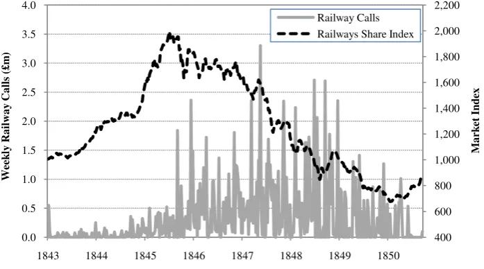
1837. Whilst the economy was weak, and these railways were being constructed, share prices

remained low and the promotion of new lines was subdued. However, between 1843 and

August 1845, railway share prices rose rapidly in a period which has become known as the

Railway Mania. Figure 1 shows several market indices, constructed by Campbell and Turner

(2010), which illustrate a pronounced rise in prices amongst all railway companies, and in the

subset of railway companies which had already been established before the Mania began.

<< INSERT FIGURE 1 >>

Several suggestions have been offered for the cause of the price changes which were

experienced at this time. Bryer (1991) has argued that the Mania could have been an attempt

to „swindle‟ investors, but this view has been challenged by McCartney and Arnold (2003).

Odlyzko (2010) has suggested that „collective hallucinations‟ were responsible for the Mania,

whilst Campbell (2010) has argued that changes in the dividends paid by the established

railways were the main cause of the price changes which occurred during this period. Despite

this research, there has been little detail provided on the new companies promoted at this

time, or on the assets which they issued.

As with some other periods of rapid asset price growth, such as the South Sea Bubble of

1720, the boom of 1825, and the Dot-Com Bubble of the 1990s, there was a substantial

increase in the promotion of new companies during the Railway Mania. The number of

railway securities listed on the London Stock Exchange underestimates the extent of

promotion, as only a small proportion ever achieved a listing, but the number of listed

securities follows the pattern in prices with a lag, as shown in Figure 2.

(7)

5

Most of the new schemes issued partially-paid shares with uncalled capital, which meant that

investors paid a small deposit and would then make future payments when the process of

construction required it. Shares issued during the Railway Mania, and throughout much of the

eighteenth and nineteenth century, were quoted with a nominal value, a par value and the

market price. The nominal value of the share was the total amount that original shareholders

were initially liable to pay to the company. The par value of the share was the amount that

shareholders had already paid to the company.

The difference between the nominal and par value reflected uncalled capital, which was the

amount that shareholders were still liable to pay to the company. Uncalled capital could be

used in several ways, with banks and insurance companies generally retaining it as a reserve,

but the railways tended to call it up in regular instalments to finance the construction of their

lines. Figure 3 illustrates the rapid increase in nominal value during the boom in railway

shares, compared to a more gradual rise in par value. This reflects the issuance of the new

securities which had only a small proportion of capital initially paid up.

Railway share prices peaked in August 1845, but fell by 18 per cent during the next three

months, just as the promotion of new railway schemes reached unprecedented levels. Many

of the railways promoted at the height of the boom never received Parliamentary

authorisation, and others faced difficulties when they began to lay their line, but the extent of

railway construction was still impressive. Estimates by Mitchell (1964) suggest that railway

investment represented 5.7 per cent of GDP in 1846, 6.7 per cent in 1847, and 4.7 per cent in

1848. However, the magnitude of railway expansion proved to be unsustainable, with the size

of investment being amongst a range of factors blamed by a Parliamentary Committee for the

(8)

6

overexpansion led several of the leading railways to announce they would not proceed with

much of the planned construction in October 1848 (Economist, November 4, 1848, p.1241). It

was not until near the end of the decade that most of the remaining construction had been

completed, and the new railways began to operate.

2 Data

Data on the number of shares in issue, the nominal value, the par value, and the market price

of every railway security listed on the London Stock Exchange between 1843 and 1850 was

obtained on a daily basis from the Railway Times, the leading railway newspaper during this

period. Data from each table, containing an average of 242.1 securities for each of the 417

weeks in the sample, was computerised and each table was then merged to produce a

comprehensive dataset. Due to the high number of listings and delistings the total number of

securities included in the dataset is 868, representing 442 railway companies.

Preference shares (88 securities) and assets issued by railways outside Great Britain and

Ireland (84 securities) were excluded. When some companies were first listed some of the

data on the number of shares, nominal value or par value were not reported. In these cases the

next reported data was assumed to be correct for the missing period. If this data was not

reported at any future period, the Railway Shareholders’ Manual (Tuck, 1845) was used to

obtain the missing details. There were 150 securities where data on either the number of

shares or par value could not be ascertained.

Several additional variables were also included. The value of uncalled capital for each asset

was calculated as the difference between the nominal value and the par value of that asset.

Data on dividends, for the subset of companies which were also reported in the Course of the

(9)

7

approximated as the yield on Consols, government debt perpetuities, which was also obtained

from the Course of the Exchange.

3 Embedded Leverage

The partially-paid shares issued during the Railway Mania were paid for in instalments. This

meant that investors subscribed to the shares for a small deposit, and then paid a fixed

amount at future dates. This feature makes them resemble future contracts, assuming that

investors could not default on their payments, or option contracts, assuming that default was

possible. One of the characteristics of these types of derivatives is the leverage which results

from their structure. Investors effectively borrow the funds from the counterparty, and obtain

exposure to the movements of the underlying asset by paying only a small initial amount. If

partially-paid shares can be modelled as derivative-like assets, then it suggests that the

leverage which results from these asset classes was available to investors during this period.

3.1 Partially-paid Shares as Futures

The relationship between fully-paid and partially-paid shares can be illustrated by a no

arbitrage argument. Investors should receive the same return from purchasing a fully-paid up

share, or from purchasing a partially-paid up share and paying the remaining liability.

Assuming that investors could not default on their liability, a partially-paid share can be

modelled as a future contract with a fixed payment in the future, and the fully-paid share can

be regarded as the underlying security, as suggested by Dale et al. (2005). Equation 1 adapts

the standard future pricing relationship, as stated by Hull (2003, p.50), to this situation and

accounts for dividends which can be expressed as a percentage of the future payment.

where: S = Price of fully-paid share, f = Price of partially-paid share,

K = Size of future payment, r = Risk-free interest rate, q = Dividend rate

(10)

8

To illustrate the implications of uncalled capital on the market price of an asset an example

will be used of the relationship between the fully-paid and partially-paid shares issued by the

Great Western Railway (GWR), before a more comprehensive analysis of other companies.

When only the market prices of the assets are compared, the difference in prices appears to

change over time, as suggested in Panel A of Figure 4. However, a fairer comparison would

be between the fully-paid „GWR Half Shares‟ and the implied price of an equivalent

fully-paid „GWR Original Share‟. This implied price can be estimated using Equation 1, by

adjusting the price of the partially-paid „GWR Original Share‟ to take account of uncalled

capital. Once these adjustments have been made, for each day of the sample between 1843

and 1850, there appears to be a close relationship between the implied prices of the fully-paid

shares, as shown in Panel B of Figure 4.

It is possible to introduce a more systematic analysis, which can be used to examine a wider

sample of companies, by testing for cointegration. By using the Engle-Granger 2-step

approach (Engle and Granger, 1987) it is possible to test if the residual from a regression

between two time series is stationary. This test for cointegration has been carried out for the

pair of GWR assets discussed above, and then repeated for all other companies which had

partially and fully paid shares listed simultaneously. To be included in the analysis a pair of

assets had to be issued by the same company, have the same pro rata dividend rights, and

both be listed on the stock market for at least one year, and be traded on average at least once

per week. Any assets which delisted and were then relisted with a different nominal or par

value were excluded. The size of the Augmented Dickey Fuller (ADF) statistic, and its

significance, for each cointegration test is shown in Table 1.

(11)

9

The results suggest that when uncalled capital is accounted for, either as a separate variable

or to produce a notional fully-paid share, there is evidence of cointegration for almost every

pair of assets. This implies that investors were pricing partially-paid shares as if they were

future contracts, which means that investors who purchased these assets were effectively

purchasing assets with embedded leverage.

3.2 Partially-paid Shares as Options

The discussion has thus far assumed that the contract which subscribers entered into to pay

future instalments was a binding obligation. However, Shea (2007b) has suggested that it

may be better to treat these assets as options, as the holder may have had the right, but not the

obligation, to pay a future amount and obtain a fully-paid share.

During the Railway Mania the legal framework for this issue was set down in the Companies‟

Clauses Consolidation Act (Parliamentary Papers, 1845, II, p.226-227). If a shareholder had

failed to pay a call two months after it was due, the company could sue the shareholder and

attempt to recover the amount due with interest, or the directors could declare the share

forfeited. At least another two months had to pass before the declaration of forfeiture could

be confirmed at a general meeting, which would allow the company to sell the forfeited

shares.

By suing shareholders the company could hope to obtain the full amount due, but they would

have to pay legal expenses. By forfeiting the share these expenses could be avoided, and the

company could sell the share in the secondary market. During the construction of the early

railways (pre-1843), the practice of forfeiting shares seems to have been preferred by at least

some of the companies. For example, the Cheltenham and Great Western Railway had

originally issued 7,500 shares, but by 1843 only 5,693 remained in issue, with the rest having

(12)

10

It should have been in the best interests of an investor to forfeit a share if the amount which

the investor was required to pay was greater than the value of that share after that payment

had been made. The default condition should therefore have been given by Equation 2.

where: S = Price of asset after payment of instalment

K = Size of instalment

(2)

By analysing data on the arrears outstanding on the instalments due on the shares of various

railway companies, taken from Parliamentary Papers (1848, LXIII, p.275-442), it is possible

to estimate whether investors chose to forfeit a partially-paid share based on the criteria given

in Equation 2. The arrears data states the amount that investors had paid on that instalment

and the amount which was still outstanding in August 1848, when the data was collected.

Alternative scenarios are considered which consider whether companies enforced forfeiture if

payment was not made after either two months, four months, one year or two years. Table 2

shows how many times the default condition was met under the various scenarios.

<< INSERT TABLE 2 >>

The results for the timeframe of four months, one year and two years suggest that there was a

significantly higher default rate when it was in the best interests of investors to default.

Although it may be inappropriate to assume that partially-paid shares were pure call options,

the difference in default rates depending on the default criteria suggests that some investors

did treat them this way.

4 Amplifying Returns

The discussion in the previous section has suggested that there is evidence that the

partially-paid shares listed during the Railway Mania were considered by investors as either futures or

(13)

11

during this period. This section will consider the impact that this leverage had on returns,

initially examining first-day returns before considering returns throughout the period.

4.1 First-day Returns

Investors who subscribed to railway IPOs were asked to pay the par value of the share as a

deposit. They would then be liable to pay calls up to the amount of the nominal value of the

shares when the company requested it. An investor who subscribed to IPOs in the primary

market and then sold those shares on the first-day that they traded on the secondary market

would receive a return given by Equation 3. The abnormal return has been calculated by

subtracting the return on that day from an index of all railway shares which has been

constructed by Campbell and Turner (2010).

where: r = Return, P = Price, Z = Par Value

(3)

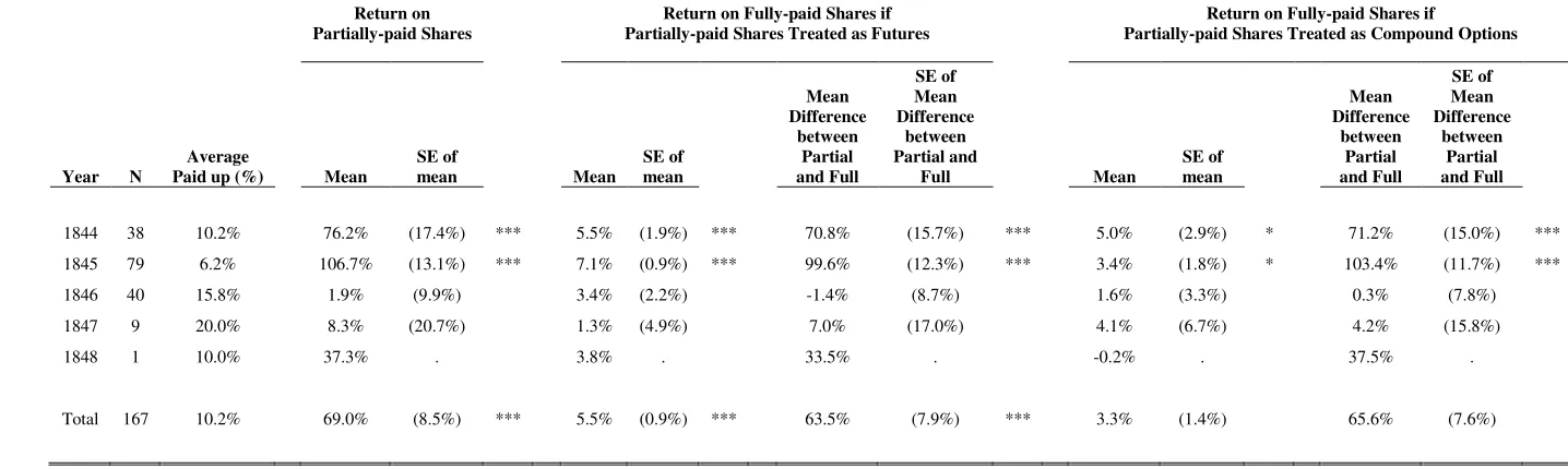
Table 3 shows that the size of the return which subscribers to new schemes could obtain

during the boom was substantial, with a mean abnormal first-day return of 76.2 per cent in

1844, and 106.7 per cent in 1845. This is consistent with commentary during the period, such

as the remark by the Railway Investment Guide (1845, p.10) that „it will be obvious that the

party who has had certain shares allotted to him, which rise to a premium (as they almost

invariably do, at least for a time) has the whole of that premium for his profit. By this means,

persons possessing only sufficient capital to pay the deposit, may more than double it in a

day‟.

If investors had been required to pay the total cost of the asset immediately, rather than in

(14)

12

be implied by adjusting the par value to include the discounted sum of future calls. The price

of the fully-paid share can be implied by adjusting the price of a partially-paid share

according to the futures pricing relationship, if it is assumed default is not possible. For this

analysis a discount rate of three per cent is used, which was close to the yield on Government

Consols, but unreported analysis suggests that similar results are obtained when other rates

are used.

where: r = Return, P = Price, Z = Par Value,

K = Size of future payment, r = Risk-free interest rate, q = Dividend rate (4)

When considering the scenario that default was possible, the price of a fully-paid share can be

implied by using an options pricing formula. Shea (2007a) has suggested modelling these

assets as n-fold compound call options. To facilitate computation for such an extensive

dataset, this paper considers them as 2-fold compound call options, and uses the closed form

formula proposed by Geske (1979). This implies that investors were initially purchasing

assets which gave them the right on the first exercise date to pay the first instalment K1, and

receive a call option which gave them the right on the second exercise date to pay the

remaining liability, K2, and receive the underlying asset. A volatility of 30 per cent has been

used for this analysis, which is close to the median volatility of 28 per cent for fully-paid

shares in the sample. Other volatilities have also been considered, although not reported, and

produce similar results.

Table 3 shows that the average returns which would have been experienced if only fully-paid

shares had been issued were just 5.5 per cent in 1844 and 7.1 per cent in 1845 if the

(15)

13

if the partially-paid share was regarded as an option contract. The difference between the

returns for partially-paid shares and fully-paid shares was substantial and significant during

these years.

These results suggest that the first-day returns for underlying ordinary shares were not

particularly high, but the return which was experienced was considerable because the full

premium was embedded in an asset on which only a small deposit was required. The impact

of uncalled capital was to magnify the first-day returns experienced by investors in new

companies. Thus the dramatic returns which investors experienced at this time from investing

in new companies were at least partially due to the effects of leverage.

4.2 Returns throughout Mania

To estimate the impact on shareholder returns throughout the Mania a similar analysis can be

repeated for each day of the sample period. If an investor subscribed to all new railway IPOs,

and then paid all subsequent calls when they were due, their cost at any particular time can be

calculated as the sum of the par values of all new companies. The market capitalisation at any

particular time reflected the price at which investors could sell their shares. Consequently, a

simple measure for estimating the return to investors was the price/par ratio. A price/par ratio

of 1 suggested that the current market price equalled the amount which had already been

invested. A price/par ratio of 2 suggested that the original investors had made a 100 per cent

return, whilst a price/par ratio of 0.5 suggested investors had lost 50 per cent of their original

investment.

The average price/par ratios for the established railways and new railways were calculated for

each day between 1844 and 1850, and are illustrated in Figure 5. The price/par ratio of the

new companies reached a peak of 2.74, which meant that an investor who had subscribed to

(16)

14

equivalent fully-paid share, when the partially-paid share is considered as a future contract,

has been calculated for each day of the sample. Alternative scenarios for the discount rate

have been employed, being -10 per cent, 0 per cent and +10 per cent. The implied price of

each equivalent fully-paid share, when the partially-paid share is treated as an option

contract, has been calculated using the approach of Geske (1979). To obtain a range of

scenarios volatilities of 20 per cent, 30 per cent and 40 per cent were analysed. The implied

total market capitalisation and the total par value for all of the new railways have been used

to calculate the implied price/par ratio for the industry, for each day, which is shown in

Figure 5.

When partially-paid shares are treated as a future contract the average price/par ratio of the

equivalent fully-paid shares of new railways reached a peak of between 1.12 and 1.18

depending on what assumptions are made about the discount rate. When partially-paid shares

are treated as option contracts, a peak of between 0.98 and 1.11 was reached, depending on

the assumptions regarding volatility. In each instance the results suggest that the returns

which investors would have experienced from investing in fully-paid shares would have been

relatively low, but due to the leveraged nature of the partially-paid shares the returns which

they actually experienced were substantial.

5 Instalment Payments

The use of leveraged derivatives also affects when investors must provide payment. Rather

than paying the full amount initially, the use of leverage makes it possible to obtain an asset

for a small initial deposit. The ability to obtain exposure to the price movements of assets

without having to immediately find the total capital required may have contributed to the

(17)

15

subscribed to the new schemes. The Economist (April 5, 1845, p.310) noted that „it is one of

their peculiar characteristics but yet not less ultimately dangerous and deceptive on that

account, that from the delay of procuring the act and getting it into operation the period when

the main bulk of capital is required is remote from that when the greatest excitement and

speculation exists, and no immediate check is therefore experienced by calls of capital.‟

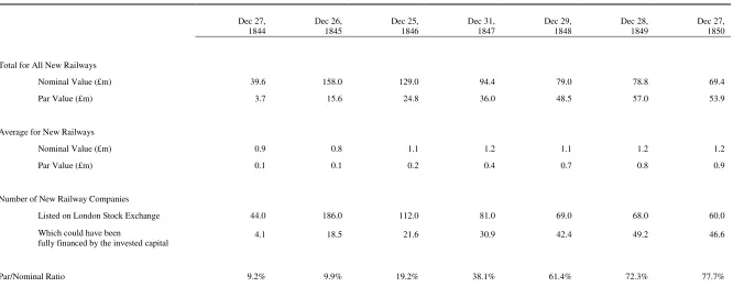
The substantial difference between the amount that investors were liable to pay (the nominal

value), and the amount which they had paid so far (the par value), is reported in Table 4 for

the end of each year. Only companies where the details of both the nominal and par values

are available are included in the analysis.

It can be seen from Table 4 that the total nominal value of new railways at the end of 1844

was £39.6m, and at the end of 1845 was £158.0m. In contrast, the total par value of these new

railways was just £3.7m in 1844, and £15.6m in 1845, which means that during the boom in

prices and promotions investors had been asked to pay up less than 10 per cent of their total

liability. This implies that although 44 new railway companies had been listed by the end of

1844, investors had only provided enough capital to fully finance 4.1 companies. By the end

of 1845, when 186 new railway companies were listed, investors had provided enough capital

to entirely finance just 18.5 companies.

When payments were eventually demanded, the resulting deleveraging may have contributed

to a decline in prices. Investors were required to make regular and sizeable payments on their

partially-paid shares during the construction phase, especially between 1846 and 1848, as

shown in Figure 6.

(18)

16

The Times (July 30, 1845, p.4) had issued warnings at the height of the Mania about the

extent and impact of future calls for capital. They said „soon or late the day will come when

an untold proportion of this year‟s scripholders will be doubly pressed, no longer able to

suffer the sums they have already paid to remain buried in the earthworks of an unfinished

line, much less to pay up the quick recurring calls of the company‟. The Economist (October

21, 1848, p.1187)noted that „every fresh call that was made upon exhausted shareholders was

attended by one of two effects – either the shares themselves upon which the call had been

made were sold in order to avoid payment, or some other shares were sold in order to raise

the money for that purpose. There was constantly an increasing number of sellers, and a

constantly diminishing number of buyers.‟ This led to the result that „lines in course of

construction in place of increasing in price as more and more capital became invested in

them, have after each new call fallen about as much as they should have risen.‟

To estimate the impact which these calls for capital had on prices, 971 changes in capital

were analysed as shown in Table 5. When a company issued a call, its return during that

week was calculated, with the abnormal return being calculated as the company return minus

the return on an index of all railway shares which has been constructed by Campbell and

Turner (2010). If an asset was not traded in the week during which the call was made the

calculation was carried out for the week that it was next traded.

An analysis of all 971 calls for capital between 1843 and 1850 suggests that a share had an

average abnormal return of -9.7 per cent in the week that a call was made on it, as shown in

Table 5. The most likely reason for the falls in prices was investors selling some shares to pay

the instalments on others. If a three week period is analysed, there was an average abnormal

(19)

17

return of -4.7 per cent. The results from these longer windows suggest that part of the decline

was temporary, reflecting the short-term difficulties which investors had in meeting the

demand for further payments. Nevertheless, there is still evidence of substantial declines

which, combined with the number of calls which were made, would suggest that this

exercised a considerable downward pressure on prices during this period. This implies that

the process of deleveraging contributed to the decline in prices during the downturn.

6 Impact on Pricing

It is possible that leverage may initially increase the demand for an asset by raising expected

returns, and by providing easier payment terms. This would suggest that the price of the asset

could be higher than it would have been if leverage was not available. However, this increase

in demand may be at least partially offset by the increased risk of the asset. It is also possible

that an increase in the price of assets could be followed by an increase in the supply of assets,

reducing the equilibrium price. The net impact of leverage on the price of an asset is thus

ambiguous.

The impact of leverage on pricing during the Railway Mania can be assessed by comparing

the prices of highly leveraged assets, namely those issued by the new railways, with other

assets. A basic approach to assessing the relative price of an asset is to compare its dividend

yield with other assets. As the new railways promoted at this time could not pay a dividend

until they had finished construction and began operation, a current dividend yield cannot be

calculated for their early stages. However, it is possible to use an approximation to calculate

what dividend they would eventually have to achieve to produce a similar return to the

non-railways and established non-railways. The dividend yield can be expressed in terms of the

(20)

18

(5)

The highest price/par ratio of the new railways from the various scenarios discussed above

was 1.18, assuming a partially paid share can be treated as a future contract, and using a

discount rate of 10 per cent. During 1845 a sample of non-railway companies were trading at

an average dividend yield of 4.5 per cent (Campbell, 2010), so to achieve a similar yield the

new railways should have been producing a dividend/par ratio of 5.3 per cent. This is a lower

bound estimate, as it does not take account of the much greater uncertainty surrounding the

new railways, or the foregone dividends during the construction phase, but it provides an

approximation for required performance.

The dividend/par ratio of the established railways peaked at 7.2 per cent during the Mania

(Campbell, 2010). An analysis of the prospectuses of 85 new railways collected from

advertisements in the Railway Times (1843-45) suggests that the promoters of these new

railways encouraged investors to expect an average dividend/par ratio of 7.9 per cent. The

lower bound estimate of the required dividend/par ratio to justify the price of the new

railways was therefore much lower than either the established railways or the prospectuses of

the new railways suggested was possible.

These calculations have been performed using the highest price/par ratio of any scenario

which has been discussed above. If a more reasonable discount rate is used, or partially paid

shares were options, then the implied dividend rate would have been even lower, suggesting

that the prices of new railway shares were not particularly high during the Railway Mania,

even at the market peak.

7 Conclusion

Using an extensive dataset, this paper has analysed the pricing of assets with uncalled capital

(21)

19

on the market at this time may be modelled as either futures or options, which implies that

investors who purchased these assets were effectively purchasing highly leveraged

derivatives.

The evidence presented above suggests that the first impact of this leverage was to amplify

the returns to investors. First-day returns for partially-paid shares were significantly higher

than the returns which investors would have received if they had only been able to purchase

fully-paid shares. The returns, throughout the boom, which were accumulated by investors in

new railways were substantially increased by the effects of leverage, but during the downturn

negative returns were also magnified.

The second impact of leverage was to allow investors to purchase assets on an instalment

payment plan. Investors could subscribe to shares in new companies for a small deposit. This

meant that although almost two hundred new railways had been listed on the market at its

peak, enough capital had been provided to finance only about twenty of them. When

payments were subsequently required, the resulting deleveraging was associated with price

declines.

The combined effects of higher expected returns, and easier payment terms, may have

increased the demand for the assets issued by the new railways. However, possibly due to the

increased risk, and the substantial increase in the supply of assets, the new railways did not

have a much higher price than the non-railways at this time.

These results suggest that leverage may play an important role in „bubbles‟. Although its

influence on prices may be limited, it affects the returns experienced by investors, and the

timing of flows of capital. The use of leverage may initially appear to be attractive to

(22)

20

investment, but it can lead to problems in a downturn, when negative returns are magnified,

and deleveraging occurs.

References

Allen, F. and Gale, D. (2000), "Bubbles and Crises", The Economic Journal, vol. 110, no. 460, pp. 236-255.

Anonymous, (1845), The Railway Investment Guide. How to Make Money in Railway Shares: A Series of Hints and Advice to Parties Speculating, British Library.

Aoki, K., Proudman, J., and Vlieghe, G. (2002). „Houses as Collateral: Has the Link between

House Prices and Consumption in the U.K. Changed?‟, Economic Policy Review,

Federal Reserve Bank of New York, May, pp. 163-77

Bernanke, B.S., and Gertler, M. (2001). 'Should Central Banks Respond to Movements in Asset Prices?' American Economic Review, vol. 91 (May), pp. 253-57.

Bryer, R. A. (1991). “Accounting for the „Railway Mania‟ of 1845–a Great Railway Swindle?”, Accounting, Organisations and Society, vol. 16, no. 5/6, pp. 439-486. Campbell, G. (2010), “Cross-Section of a „Bubble‟: Stock Prices and Dividends during the

British Railway Mania”, SSRN Working Paper.

Campbell, G. and Turner, J. (2010), “„The Greatest Bubble in History‟: Stock Prices during the British Railway Mania”, SSRN Working Paper.

Dale, R., Johnson, J.E.V. and Tang, L. (2005), „Financial Markets can Go Mad: Evidence of

Irrational Behaviour during the South Sea Bubble‟, Economic History Review, vol.

58, no. 2, pp. 233-271.

Detken, C. and Smets, F. (2004), 'Asset Price Booms and Monetary Policy', ECB Working Paper no. 364.

Engle, R. F. and Granger, C.W.J. (1987), „Co-Integration and Error Correction:

Representation, Estimation, and Testing‟, Econometrica, vol. 55, pp.251-276.

Economist (2008). The Beauty of Bubbles, December 18.

Geithner, T. (2010), „Remarks before the American Enterprise Institute on Financial

Reform‟, Speech at the American Enterprise Institute, March 22.

Geske, R. (1979), „The Valuation of Compound Options‟, Journal of Financial Economics, vol. 7, pp. 63-81.

Guiso, L., Sapienza, P. & Zingales, L. (2009), „Moral and Social Constraints to Strategic

Default on Mortgages‟, CEPR Working Paper.

(23)

21

Kindleberger, C.P. (2000), Manias, Panics, and Crashes: A History of Financial Crises, John Wiley & Sons.

Lewin, H.G. (1968), The Railway Mania and its Aftermath, 1845-1852 (Being a Sequel to Early British Railways), Rev. Edn, A. M. Kelley.

MacDermot, E.T. (1964), History of the Great Western Railway, Ian Allan Ltd. McCartney, S. and Arnold A. J. (2003). “The Railway Mania of 1845-1847: Market

Irrationality or Collusive Swindle Based on Accounting Distortions?”Accounting, Auditing and Accountability Journal, vol. 16, no.5, pp.821-52.

Mitchell, B.R. (1964), „The Coming of the Railway and United Kingdom Economic Growth‟,

Journal of Economic History, vol. 24, no. 3, pp. 315-336.

Nairn, A. (2002), Engines that Move Markets: Technology Investing from Railroads to the Internet and Beyond, Wiley.

Odlyzko, A. (2010). Collective Hallucinations and Inefficient Markets: The British Railway Mania of the 1840s, University of Minnesota.

Parliamentary Papers (1847-48), LXIII, p.275-442 „Return of the names of railways for which acts have been obtained; calls made; amount received and remaining due; sums borrowed which remain owing; balance of capital uncalled for, and of money which the companies retain power to borrow; and, periods for which the companies have postponed making further calls.‟

Parliamentary Papers (1847-48), VIII, Pt. I, p.1, „Reports from the Secret Committee on Commercial Distress; with an Index‟.

Pollins, H. (1971), Britain's Railways: An Industrial History, David and Charles (Publishers) Limited.

Shea, G.S. (2007a), „Understanding Financial Derivatives During the South Sea Bubble: The

Case of the South Sea Subscription Shares‟, Oxford Economic Papers, vol. 59, no.

Supplement 1, pp. i73.

Shea, G.S. (2007b), „Financial Market Analysis Can Go Mad (in the Search for Irrational

Behaviour During the South Sea Bubble)‟, Economic History Review, vol. 60, no. 4,

pp. 742-765.

Simmons, J. (1978), The Railway in England and Wales, 1830-1914, vol.1, Leicester University Press.

(24)

[image:24.595.121.468.121.327.2]

22

Figure 1: Weekly Market Indices of All Railways, Established Railways and Non-Railways, 1843-50

Source: Campbell and Turner (2010).

Notes: Railway share indices calculated from weekly share price tables in Railway Times (1843-50). Non-Railway share index calculated from weekly share price tables in Course of the Exchange (1843-50). The All-Railway index includes all railway securities, whereas the Established-Railway index includes those railways which were operating before January 1843. The Non-Railway index includes the twenty largest non-railways by market capitalization. Capital gains for each company are weighted by market capitalization to produce weekly market indices.

400 600 800 1,000 1,200 1,400 1,600 1,800 2,000 2,200

1843 1844 1845 1846 1847 1848 1849 1850

In

d

ex

L

ev

el

(25)

[image:25.595.123.474.119.315.2]

23

Figure 2: Number of Railway Securities Listed on London Stock Exchange, and Railway Share Index 1843-50

Notes: Railway share index and number of securities listed on London Stock Exchange calculated from weekly share price tables in Railway Times (1843-50). Market index constructed from market returns, which have been calculated by weighting the returns of the component companies by their market capitalisation at the start of the day.

400 600 800 1,000 1,200 1,400 1,600 1,800 2,000 2,200 0 50 100 150 200 250 300 350

1843 1844 1845 1846 1847 1848 1849 1850

Ma rk et Inde x N u m b er o f S ec u ri ti es

Railway Securities listed on LSE

(26)

[image:26.595.123.466.146.345.2]

24

Figure 3: Total Par Value and Nominal Value of Railway Shares Listed on London Stock Exchange, 1843-50

Notes: Nominal Value and Par Value for each company listed on London Stock Exchange obtained from weekly share price tables in Railway Times (1843-50). Industry Nominal and Par Values calculated by summing individual companies.

0 50 100 150 200 250 300

1843 1844 1845 1846 1847 1848 1849 1850

N

o

m

in

a

l/

Pa

r

V

a

lu

e

(£

m

il

li

o

n

s)

Nominal Value

(27)

[image:27.842.437.770.171.383.2]

25

Figure 4: Daily Share Prices of a GWR Full Share and Two Half Shares, 1843-50

Panel A: Prices Observed in Market Panel B: Prices Adjusted for Uncalled Capital Discounted at Actual

Risk-Free and Dividend Rates

Notes: Share prices obtained on a daily basis from weekly share price tables in Railway

Times (1843-50).

Notes: Share prices and par values obtained from weekly share price tables in Railway

Times (1843-50). Implied price of a GWR original share calculated using Equation 1.

£0 £50 £100 £150 £200 £250 £300

1843 1844 1845 1846 1847 1848 1849 1850

Sha

re

P

ri

ce

(£

)

GWR Original Share

GWR Half Share (x2)

£0 £50 £100 £150 £200 £250 £300

1843 1844 1845 1846 1847 1848 1849 1850

Sha

re

P

ri

ce

(£

)

GWR Original Share [Price + Ue(-r+q)t]

(28)

[image:28.842.442.771.151.355.2]

26

Figure 5: Price/Par Ratio of New Railways, 1844-50

Panel A: Shares Treated as Futures, using Alternative

Scenarios of Discount Rate

Panel B: Shares Treated as Compound Call Options, using Alternative Scenarios of Volatility

Notes: Implied market capitalisation and par value calculated for individual new railways, promoted after 1843, using alternative scenarios of the interest and dividend rates. Implied price/par ratio of all new railways calculated as implied total market price/total cost.

Notes: When treated as a future the implied price/par ratio calculated as total price/total cost using an interest rate of 3 per cent and dividend rate of 0 per cent to discount uncalled capital. When treated as an option the price of a partially-paid share is assumed to be the price of a compound call option, using alternative assumptions about volatility. The pricing formula for a compound call option (Geske, 1979) was used to imply the price of an underlying fully-paid share for each company.

0.0 0.5 1.0 1.5 2.0 2.5 3.0

1844 1845 1846 1847 1848 1849 1850

Pr ic e/ Pa r R a ti o Market Price/Par

Implied from Future Pricing (-r+q = -0.1) Implied from Future Pricing (-r+q = 0) Implied from Future Pricing (-r+q = 0.1)

0 0.5 1 1.5 2 2.5 3

1844 1845 1846 1847 1848 1849 1850

Pr ic e/ Pa r R a ti o Market Price/Par

Implied from Future Pricing

(29)

[image:29.595.121.470.158.352.2]

27

Figure 6: Weekly Railways Calls and Railway Share Index 1843-50

Notes: Railway share index and volume of calls calculated from weekly share price tables in Railway Times

(1843-50). 400 600 800 1,000 1,200 1,400 1,600 1,800 2,000 2,200 0.0 0.5 1.0 1.5 2.0 2.5 3.0 3.5 4.0

1843 1844 1845 1846 1847 1848 1849 1850

(30)

[image:30.842.35.823.149.445.2]

28

Table 1: Augmented Dickey-Fuller (ADF) Tests of Residual from Estimated Cointegrating Relationships between Fully-paid and Partially-paid Shares of Established Railway Companies

Variables Included in Cointegrating Relationship

Y = PriceF

X1 = PriceP

Y = PriceF

X1 = PriceP

X2 = UncalledP

Y = PriceF

X1 = PriceP

X2 = UncalledP

X3 = Rf

X4 = Div

Y = PriceF

X1 = PriceP + Ue(-r+q)t, where (-r+q) is equal to:

Fully-paid Share

(Y = PriceF)

Partially-paid Share

(X = PriceP) Actual -10% 0% 10% Obs

Edinburgh and Glasgow Half Shares -1.60 -4.78 *** -5.33 *** -4.33 *** -3.59 ** -4.13 *** -4.72 *** 1,186 Great Western Half Share Full Shares -3.82 ** -16.36 *** -16.82 *** -14.50 *** -8.67 *** -13.21 *** -12.04 *** 2,284 Great Western Half Share Fifth Shares -3.79 ** -17.83 *** -18.26 *** -15.93 *** -10.09 *** -14.21 *** -17.20 *** 2,270 Great Western Half Share Sixth Shares -1.13 -9.83 *** -10.18 *** -8.90 *** -6.78 *** -8.29 *** -9.75 *** 1,119 Great Western Half Share Quarter Shares -2.38 -13.28 *** -13.18 *** -11.91 *** -9.31 *** -11.61 *** -11.23 *** 1,379 London and North Western New Shares -0.87 -7.52 *** -8.64 *** -8.17 *** -2.94 -6.18 *** -6.11 *** 1,050 London and North Western Fifth Shares -1.27 -9.07 *** -10.79 *** -6.11 *** -5.69 *** -7.07 *** -4.07 *** 1,359 London and North Western Quarter Shares -1.47 -6.25 *** -6.55 *** -5.03 *** -4.74 *** -4.91 *** -5.04 *** 537 Midland Half Shares -1.43 -5.03 *** -5.72 *** -4.34 *** -3.35 * -4.23 *** -4.02 *** 1,284

Midland New Shares -2.02 -8.84 *** -9.24 *** -8.45 *** -5.67 *** -8.27 *** -6.65 *** 989

York and Newcastle New Shares -2.70 -6.85 *** -6.79 *** -6.37 *** -6.65 *** -6.65 *** -6.07 *** 327 York, Newcastle and Berwick Extension No. 1 Shares -2.51 -12.00 *** -12.04 *** -9.92 *** -7.04 *** -9.04 *** -10.55 *** 1,008 York, Newcastle and Berwick Extension No. 2 Shares -1.93 -6.90 *** -7.58 *** -5.19 *** -3.47 ** -4.70 *** -5.23 *** 438 York and North Midland Half Shares -4.95 *** -14.35 *** -14.51 *** -12.30 *** -10.86 *** -11.67 *** -12.59 *** 1,279 York and North Midland E&W Riding Shares -0.89 -5.94 *** -7.86 *** -3.82 ** -2.95 -3.31 * -4.20 *** 1,035 York and North Midland Extension Shares -1.54 -4.97 *** -7.40 *** -2.61 -1.42 -2.00 -2.95 886 York and North Midland Scarborough Branch Shares -3.31 * -4.27 ** -4.31 * -2.90 -2.96 -2.92 -2.90 870

(31)

[image:31.842.213.628.244.373.2]

29

Table 2: Forfeiture Rates on Railway Share Instalments, using Alternative Scenarios for Deadline on Payment

Time between Instalment Due Date and Deadline for Payment

Criteria Met Forfeiture Rate

Difference in Forfeiture Rates

SE of Difference

N S-K>=0 S-K<0 S-K>=0 S-K<0

2 Months 225 214 11 10.5% 13.6% 3.2% (4.1%)

4 Months 221 197 24 8.5% 19.0% 10.5% *** (2.4%)

1 Year 163 132 31 5.5% 14.8% 9.3% *** (1.8%)

2 Years 74 52 22 2.7% 6.3% 3.5% ** (1.7%)

(32)

[image:32.842.50.768.156.371.2]

30

Table 3: New Railways’ First-day Abnormal Returns

Return on Partially-paid Shares

Return on Fully-paid Shares if Partially-paid Shares Treated as Futures

Return on Fully-paid Shares if

Partially-paid Shares Treated as Compound Options

Year N

Average

Paid up (%) Mean

SE of

mean Mean

SE of mean Mean Difference between Partial and Full SE of Mean Difference between Partial and

Full Mean

SE of mean Mean Difference between Partial and Full SE of Mean Difference between Partial and Full