A Defense against Malicious Attackers Using Machine Learning Algorithm in Wireless Sensor Networks

© 2016, IRJET ISO 9001:2008 Certified Journal

Page 484

A Defense against Malicious Attackers Using Machine Learning

Algorithm in Wireless Sensor Networks

Nisha Vijayan

_{, Kishore Sebastian}

1

_{Student, Dept of Computer Science & Engineering, St Joseph’s college of Engineering & Technology, Palai, Kerala,}

India

2

_{Assistant Professor, Dept of Computer Science & Engineering, St Joseph’s college of Engineering & Technology,}

Palai, Kerala, India

---***---Abstract -

deploy are highly vulnerable to attacks. There are many defensive measures taken. Mostly the measures taken allow the attack to take place and then analyze with past reading of the sensor nodes with current reading. However, this consumes lots of energy and also some attacks cannot be detected here. This paper introduces an energy efficient, fault tolerant machine learning algorithm. This is an opportunistic machine learning algorithm that incorporates machine learning in it. In machine learning the nodes decide whether to accept packets from certain nodes based on threshold value.

Key Words: Wireless Sensor Networks, machine learning, optimization, routing.

1.

INTRODUCTION

Some attacks in wireless sensor networks cannot be easily detected using the usual anomaly detection methods. Moreover, it consumes a lot of energy. As, the attack is allowed to take place initially and then other nodes have to be infected. Then the final result is compared with the past readings. Depending on the variation in the readings it is decided which node is malicious. In the proposed system this process is changed such that whenever an attack takes place it is detected and it is not allowed to infect other nodes.

The routing methodology used here is opportunistic routing. I.e. the best path is decided using certain calculations and the path can be switched depending on the situation. For the decision making in this system machine learning is used. i.e. the nodes decide whether to accept packets from a certain node or not, rather than the broadcasting methodology which would again consume energy and resources.

1.1 Current System

In the study done, the authors have detected the malicious nodes in the network using the Opportunistic Routing in Presence of Malicious Nodes. The behavior of

the nodes present in the network are analyzed and if there is selfish occurring in the network from the past observed patterns, then the nodes are detected.

For example, first the performance of the nodes will be analyzed using the parameters say number of control packets. Then the nodes will be analyzed under the attack. During the attack the nodes will have flood the route request packets in the network. And the number of control packets flooded in the network will be significantly increased.

The anomaly based method will compare the current results with the past patterns. When the anomaly is found, the malicious node is detected in the network.

1.2 Proposed System

The main aim of this work is to detect the malicious node attacks in the network and thereby prevent them so that resources in the network can be saved. Concept of machine learning is used to detect the malicious node. Here the nodes are trained with a set of decisions that needs to be performed before taking any action.

© 2016, IRJET ISO 9001:2008 Certified Journal

Page 485

2. THE CONCEPT OF MACHINE LEARNING

Learning automata is a self operating learning model. Here, “learning” refers to the process of gaining knowledge during the execution of a simple machine code (automation), and using gained knowledge to decide on action to be taken in the future. This model has three main components- the automation, the environment and the reward/penalty structure. The Automaton refers to the self-learning machine. Environment is the medium in which this machine functions. The Automaton continuously performs actions on the Environment and the Environment responds to these actions. This response may be either positive or negative which serves as the feedback to the Automaton, this leads to the Automaton either getting rewarded or penalized. Gradually, the Automaton learns the characteristics of the Environment and identifies “optimal” actions that can be performed on the Environment.

2.1 Automation

The Learning Automaton can be represented as a quintuple represented as {Q, A, B, F, H}, where :

• Q: is the finite set of Internal States Q = {q1, q2,

q3, . . . , qn} where qn is the state of the

automaton at instant n.

• A: is a finite set of actions performed by the automaton. A = {α1, α2, . . . , αn} where αn is the action performed by the automaton at instant n.

• B: is a finite set of responses from the environment. B = {β1, β2, β3, . . . , βn} where βn

is the response from the environment at an instant n.

• F: is a mapping function. Maps the current state and input to the next state of the automaton. Q×B →Q.

• H: is a mapping function. Maps the current state and response from the environment to determine the next action to be performed.

2.2 Environment

The Environment refers to the medium in which the Automaton functions. An Environment can be abstracted by a triple {A, B, C}. A, B as defined in Sect. 1, C is defined as follows. C = {c1, c2, . . . , cr } is a set of penalty probabilities, where element ci ∈C corresponds to an input action αi. We now provide a few important definitions used in the field of LA. Given an action probability vector P(t) at time ‘t ’, the

average penalty, M(t), is defined as :

M(t) = E [β(t)|P(t)] = Pr [β(t) = 1|P(t)]

=∑ r × Pr[α(t) = αi] =∑

The average penalty for pure chance automation is given by:

∑

As t→∞, if the average penalty M(t)<M0, at least asymptotically, the automaton is generally considered to be better than the pure-chance automaton. E[M(t)] is given by:

E[M(t)] = E {E [β(t)|P(t)]} = E[β(t)].

2.3 System Model

2.3.1 Network Model

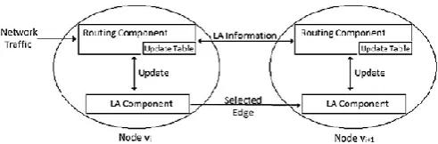
An ad hoc network is represented using a graph W = (V ,E), where V represents the set of vertices and E the set of edges. The vertices are the nodes in the network and the edges are the links in between the nodes. A path is a set of vertices connected to each other from a vertex (which can also be source) to destination. Faults can occur unpredictably in any node in the network. It is assumed that all links in the network are bidirectional, i.e., if (vi, vi+1)→E, then (vi+1, vi )→E also exists. Each node ‘v’ has two components: a routing component and an LA component. Each node’s LA component functions independently of others and shares updates through an update table maintained at the routing component which shares LA information through the neighbor nodes. As shown in Fig. 1, the LA component shares the information across the neighboring node to learn about the network. The proposed protocol is dependent on the routing protocol, but not on the network topology.

Interactions between the different components of a node and its neighboring node are shown in Fig-1.

Fig-1: Interactions between different components of a node and its neighboring node.

2.3.2 Learning Automation Model

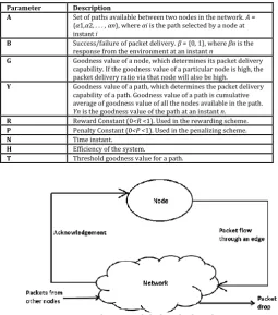
In the proposed model, an LA is associated to each node in the Wireless Sensor Network. Each LA component has the parameters described in Table 1.

© 2016, IRJET ISO 9001:2008 Certified Journal

Page 486

Table -1: LA parameters

Parameter Description

A Set of paths available between two nodes in the network. A =

{α1,α2, . . . , αn}, where αi is the path selected by a node at instant i

B Success/failure of packet delivery. β = {0, 1}, where βn is the

response from the environment at an instant n

G Goodness value of a node, which determines its packet delivery

capability. If the goodness value of a particular node is high, the packet delivery ratio via that node will also be high.

Y Goodness value of a path, which determines the packet delivery

capability of a path. Goodness value of a path is cumulative average of goodness value of all the nodes available in the path. Yn is the goodness value of the path at an instant n.

R Reward Constant (0<R <1). Used in the rewarding scheme.

P Penalty Constant (0<P <1). Used in the penalizing scheme.

N Time instant.

H Efficiency of the system.

T Threshold goodness value for a path.

Fig-2: Learning update model for fault-tolerant routing protocol.

3. BASIC COMPONENTS OF LAFTRA- LEARNING

AUTOMATA BASED FAULT TOLERANT ROUTING

ALGORITHM

3.1 Goodness value table

In this approach, the LA component maintains a goodness table at each node. The table contains the goodness value of all paths from the node to the destination node. The table consists of the entries as shown in Fig. 3. The entry NODE contains the destination node. NEXT HOP contains the neighboring node which is part of the path with highest goodness value to the destination node from the given node. UPDATE SEQUENCE NUMBER is used to keep track of the updates in the table. The table is updated only if an update message with higher update sequence number than the current update sequence number arrives. PATH_GOODNESS contains the goodness value of the best path from the current node to the destination and calculated on the basis of reward/penalty scheme in Sects. 3.3 and 3.4.

.

3.2 Goodness Update Message

The update message sent by the neighboring nodes about the goodness value of the path should be small in size, in order to minimize the network overhead, and should be sent on a regular basis in order to avoid redundant entries. We propose a new goodness update message header which will inform the neighboring node about a particular node’s goodness value.

Goodness value table gets updated by update messages which will be sent by the node to its neighbors either during route reply message or during packet acknowledgment. This way the goodness value table remains updated and no redundant information is stored in it.

3.3 Reward Scheme

The LA at each node will apply a rewarding scheme on successful packet delivery.

LA will reward the node in the following manner:

Reward Function

if (current node = destination)

G = G×P;

Y = G;

else if(Y<T)

G = G + R

Y= η *G+(1- η)*Y η -1

Else

G=G+R

Algorithm -1: Reward Function

© 2016, IRJET ISO 9001:2008 Certified Journal

Page 487

3.4 Penalty Scheme

The LA will penalize the node if there is a packet delivery failure in the following manner:

Penalization Function

if (current node = destination)

G = G×P;

Y = G;

else

G = G + R

Y= η *G+(1- η)*Yη -1

Algorithm -2: Penalization Function

Here, η is similar to reward scheme. Here, each node rewards or penalizes the path from itself to destination. Mobile nodes existing in the network make up the environment. LA at each node rewards or penalizes the node based on packet delivery. The value of P should be around 0.3–0.5 which decreases the goodness value to about half on every packet delivery failure. If the value of P

is too low, then the source will continue to use the path till long after a fault occurs in the network. If the value of P is too high, the network will not tolerate even the accidental packet failure.

4. PROPOSED ALGORITHM IN STEP BY STEP

APPROACH

1. Deploy all the nodes in the network. 2. Select source and destination node.

3. Initialize machine learning parameters. HOW Machine learning parameters are initialized the same as variables are declared in c language. 4. In machine learning, the number of neighbors the

nodes has in the network will be found and find maximum number of neighbors that a node has. We here refers to learning automata system. 5. Then we set the threshold value equal to

maximum number of neighbors calculated in the previous step plus some constant value. This is done because normally a node will forward one single request packet to its neighbor node. And the total number of packets that a node can forward can never be more than the threshold value.

6. If the total number of route request packets forwarded by the node to its neighbors during the route request phase is less than threshold value then the node will be rewarded with one credit point.

7. If the total number of route request packets forwarded by the node to its neighbors during the route request phase is more than the threshold value then the node will be assigned penalty points.

8. At the end of the route request phase, the goodness value of each node will be calculated. 9. Goodness values = G +R. for node that is rewarded. 10. Goodness values = G * P for node that is penalized. 11. Source node starts forwarding the route request

packets to its neighbor nodes. If neighbor nodes has route to the destination node then they will reply back to the source otherwise they will forward the route request to their neighbors. 12. The goodness value of all the paths will be

calculated.

13. The destination node will chose the path having the highest goodness value. If any path contains the attacker node that is flooding the network then it will be penalized and that path will automatically have less goodness value.

14. Now the destination node will know which path has very less goodness value, it will detect the lower goodness value path.

So the path will not be chosen then the attack will be prevented.

5. SIMULATION AND RESULTS

In order to evaluate the performance of the proposed protocol, extensive simulation studies has been conducted using the ns-2 for 30 independent runs with 95% of confidence.

© 2016, IRJET ISO 9001:2008 Certified Journal

Page 488

Fig -3: Network Topology.

Fig -4: Communication between Networks.

Fig -5: Malicious unable to attack other nodes.

4.1 Evaluation of Results

The output comparing with existing system is based on four factors, as follows:

 Inter sensor delay  Transmission overhead  Packet Loss

 Packet delivery ratio

A comparative study has been made and the results are plotted in graphs. On evaluating the results the performance of proposed system is higher compared to proposed system. The graph is plotted based on increasing number of malicious nodes. This shows that how well the

proposed algorithm could work on increasing number of malicious nodes.

Chart -1: Graph for average delay X-Axis: Number of malicious nodes

Y-Axis: Average inter sensor delay in seconds

AverageSensorDelay = Total PacketTransfer Time/Total no: of ReceivedPackets

On applying algorithm the average inter sensor delay could be reduced. The red line in the graph indicates the proposed system and the green line indicates existing systems.

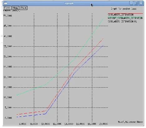
Chart -2: Graph for packet loss X-Axis: Number of malicious nodes Y-Axis: Packet loss in percentage

© 2016, IRJET ISO 9001:2008 Certified Journal

Page 489

The red line in the graph indicates the proposed system and the green line indicates existing systems.

Chart -3: Graph for packet delivery ratio

X-Axis: Number of malicious nodes

Y-Axis: Packet Delivery Ratio in Percentage

PacketDeliveryRatio = (Total Packets Sent/Total Packets Recieved) *100

On applying algorithm the packet delivery ratio could be increased. The red line in the graph indicates the proposed system and the green line indicates existing systems.

3. CONCLUSIONS

A study was made on attacks that could affect the efficiency of the wireless sensor networks. This lead to the introduction of learning automata based fault tolerant algorithm. A detailed description of learning automata is shown. Also how it is incorporated in the opportunistic routing algorithm has also been described. It is also explained how attacks could be avoided using this methodology. Further, the efficiency of this algorithm could be compared with the other existing routing and anomaly detection algorithms.

REFERENCES

[1] Salem N, Hubaux J-P (2006) Securing wireless mesh networks. IEEE Wirel Commun 13(2):50–55. doi:10.1109/MWC.2006.1632480.

[2] Akyildiz I,Wang X,WangW(2005)Wireless mesh

networks: a survey. Comput Netw 47(4):445–487. doi:10.1016/j.comnet.2004.12.001.

[3] Yi P, Tong T, Liu N, Wu Y, Ma J (2009) Security in wireless mesh networks: challenges and solutions. In: Sixth international conference on information technology new generations, ITNG ’09, 27–29 April, pp 423–428. doi:10.1109/ITNG.2009.20.

[4] Glass S, PortmannM, Muthukkumarasamy V (2008) Securing wireless mesh networks. IEEE Internet Comput 12(4):30–36. doi:10.1109/MIC.2008.85. [5] Xue Y, Nahrstedt K (2004) Providing fault-tolerant ad

hoc routing service in adversarial environments. Wirel Pers Commun 29(3–4):367–388.

[6] Xue Y, Nahrstedt K (2003) Fault-tolerant routing in mobile ad hoc networks. In: Wireless communications and networking, 2003, WCNC, 20–20 March, vol 2, pp 1174–1179. doi:10.1109/WCNC. 2003.1200537. [7] Royer EM, Toh C-K (1999) A review of current routing

protocols for ad hoc mobile wireless networks. IEEE Pers Commun 6(2):46–55. doi:10.1109/98.760423. [8] Narendra KS, Thathachar MAL (1974) Learning

automata: a survey. IEEE Trans Syst Man Cybern SMC-4(4):323–334. doi:10.1109/TSMC.1974.5408453.