1844
PARALLEL K-MEANS FOR BIG DATA: ON ENHANCING
ITS CLUSTER METRICS AND PATTERNS
VERONICA S. MOERTINI1, LIPTIA VENICA2
1,2
Informatics Department
Parahyangan Catholic University
Bandung – Indonesia
Email: [email protected], [email protected]
ABSTRACT
K-Means clustering algorithm has been enhanced based on MapReduce such that it works in distributed Hadoop cluster for clustering big data. We found that the existing algorithm have not included techniques for computing the cluster metrics necessary for evaluating the quality of clusters and finding interesting patterns. This research adds this capability. Few metrics are computed in every iteration of k-Means in the Hadoop’s Reduce function such that when it is converged, the metrics are ready to be evaluated. We have implemented the proposed parallel k-Means and the experiments results show that the proposed metrics are
useful for selecting clusters and finding interesting patterns.
Keywords: Clustering Big Data, Parallel k-Means, Hadoop MapReduce
1.INTRODUCTION
The high utility of IT and the Internet by individuals as well as organizations have produced big data in recent years. Big data comes from various sources, such as sensor equipment, social media, website logs, clicks, and stored with either unstructured, semi structured or structured format. With the availability and accessibility of these data, analyzing them using data mining techniques, such as clustering, for obtaining valuable information has become a necessity in organizations.
The emerging technology Hadoop with its MapReduce components have been developed for analyzing big data in a distributed computing environment. Hadoop offers few advantages, the one that is beneficial to small organizations is the machines in the distributed network can be just commodity computers [1]. A MapReduce program must processes data by manipulating key-value pairs and produce some other form of key-value pairs designed by developers. With this strict scheme, the “traditional” data mining techniques, such as k-Means algorithm, should be enhanced such that it works in the Hadoop environment.
A good clustering method will produce high quality clusters with high intra-class similarity and low inter-class similarity. It should also be able to discover the valuable hidden patterns [2,3].
We have found two parallel k-Means developed for Hadoop environment discussed in [4] and [5] (see Subsection 2.4). Both enhanced k-Means
consist of Map and Reduce algorithms and functions that do the k-Means computations. However, these algorithms have not computed sufficient metrics that are necessary for evaluating the clusters quality and valuable patterns.
Issues of evaluating the cluster quality: It is
known that k-Means takes k (number of clusters) as
one of its inputs. Finding the best k requires trial and
error by examining and evaluating the clusters based on few metrics such as the size of each cluster, cohesion of the clusters, and separation of the clusters [3]. Thus, parallel k-Means should also compute these metrics such that the clusters quality can be evaluated.
Issues of discovering the valuable hidden patterns or knowledge from dataset: By taking
inputs of dataset and k, k-Means then produces
centroids of all cluster and labels each object in the dataset with its cluster number. The centroids can be used as a pattern metric. However, by using only the centroids, interesting patterns or knowledge may not be identified correctly/completely. Addressing this need, [3] have defined few other cluster pattern metrics, such deviation, minimum, maximum of object attribute values, and number of objects in each cluster. Hence, these metrics should also be computed in the parallel k-Means.
1845 previously developed parallel k-Means to compute
these metrics efficiently in the distributed
environment? Once the algorithm has been enhanced, how to use this for obtaining interesting patterns from big data?
In this research, we enhance the parallel k-Means to address those issues and conduct experiments using two sample of big data for obtaining knowledge. Our main contribution is enhancing the previously developed parallel k-Means based on MapReduce such that it has the capability to generate the necessary metrics for evaluating clusters quality and discovering interesting patterns.
This paper presents some related literature review, proposed techniques, experiment results using two big dataset, conclusion and further works.
2.LITERATURE REVIEW
2.1. Clustering Stages
Among business organizations, data mining techniques are commonly used in supporting customer relationship management. The cycle of using data mining include stages of identifying the
business problem, mining data to transform the data into actionable information, acting on the information, measuring the results [6]. When the problem is lack of data insights, data miners can define the objective as to obtain knowledge from the data and select clustering technique to seek solutions. The processes for clustering data is shown in Fig. 1. Based on the objective, data miner should gather and select some raw data. Then, the selected dataset should be preprocessed that may involve data cleaning, attribute selection and transformations [3]. Data cleaning needs to be performed as raw dataset may contain missing values, outliers or unwanted values. Some attributes may be irrelevant such that these should be removed. Attribute values may need to be normalized or transformed into the certain values and/or types that are accepted by the algorithms. The patterns resulted from clustering are then evaluated by some measures to obtain knowledge, which can be used to design organizational actions.
raw dataset pre-processed clustering algorithm patterns evaluation knowledge Figure.1: Knowledge Discovery Process [7].
2.2. k-Means Algorithm, Cluster Quality and Patterns Generation
Clustering aims to find similarities between data objects according to the characteristics found in the objects and grouping similar objects into clusters [2]. As k-Means algorithm processes matrix data input where all of the attributes must be numeric, each object is a vector.
The k-means algorithm partitions a collection of n vector xj, j = 1,…,n into c groups Gi, i = 1,…,c,
and finds a cluster center (centroid) in each group such that a cost function of dissimilarity measure is minimized([8] as appeared in [9, 11]). If a generic distance function d(xk,ci) is applied for vector xk in
group i, the overall cost function is
∑
∑ ∑
= = ∈ − = = c i ci kxkGi i k
i d x c
J J
1 1 ,
. ) (
(1)
The partitioned groups are represented by an c x
n binary membership matrix U, where element uij is
1 if the jth data point xj belongs to group i, and 0
otherwise. The cluster center (centroid) ci is the
mean of all vectors in group i:
∑
∈=
i k k i i G x kx
G
c
,|
|
1
(2)where |Gi| is the size (object numbers) of Gi.
The k-means algorithm is presented with a dataset xi, i = 1,…,n. The algorithm determines the
centroid ci and the membership matrix U iteratively
using the following steps: (1) Initialize the cluster
center ci, i = 1,…,c; (2) Determine the membership
matrix U; (3) Compute the cost function by Eq. (1). Stop if its improvement over previous iteration is below a certain threshold or maximum iteration (defined by data miners) is reached; (4) Update the cluster center by Eq. (2). Go to step 2.
The performance of the k-means algorithm depends on the initial positions of the cluster centers. k-Means is relatively efficient with O(tkn), where n is total vectors/objects, k is the cluster numbers, and t is the iterations. Normally, k, t << n.
Measuring Clustering Algorithm Quality: A good clustering method will produce high quality clusters with high intra-class similarity and low inter-class similarity. It should also be able to discover the hidden patterns [2]. Other requirements are: (1) Scalability; (2) Able to deal with noise and outliers; (3) Interpretability and usability, etc.
1846 To achieve this, data miners should assess the homogeneity or cohesion of the clusters and the level of similarity of their members, as well as their separation.
In examining and evaluating the clusters, [3] proposes 3 measures:
(a) The number of clusters and the size of each cluster: A large, dominating cluster which concentrates most of the records may indicate the need for further segmentation. Conversely, a small cluster with a few records merits special attention. If considered as an outlier cluster, it could be set apart from the overall clustering solution and studied separately.
(b) Cohesion of the clusters: A good clustering solution is expected to be composed of dense concentrations of records around their centroids. Two metrics can be calculated to summarize the concentration and the level of internal cohesion of the revealed clusters, which are:
(b.1) Standard deviations of cluster attributes and pooled standard deviations of each cluster:
Standard deviations of the attribute j in a cluster can
be defined as:
(3) where xi is the attribute value of object i, µ is the
average of this attributes, N is the total object
members in the corresponding cluster.
The pooled standard deviation of a cluster
having k attributes and N object members can be
defined as:
∑
(4)
(b.2) Average of squared Euclidean distances (SSE) between the object and their centroid as follows:
∑ ∑&() () !" #, %& '
(5)
where Ci is the centroid of cluster i, x is an
object of cluster i, and N is the total objects.
(c) Separation of the clusters: High clusters should have low inter-cluster similarity or high inter-cluster dissimilarity. This can measured by computing the silhouette coefficients of the clustering results.
The silhouette coefficient of each clustered object, S(i), is computed as:
))
(
),
(
max((
))
(
)
(
(
)
(
i
b
i
a
i
a
i
b
i
S
=
−
(6)
where a(i) = average dissimilarity between
object i and all other objects of the cluster to which i
belongs and b(i) = average dissimilarity between
object i and its “neighbor” cluster (the nearest
cluster to which i belongs). In Eq. 6, 0 ≤ S(i) ≤ 1.
Large value of S(i) denotes that object i is well clustered, small value denotes the opposite and
negative value of S(i) denotes that object i is
wrongly clustered. Generally if the average of S(i)
for all clustered objects is greater than 0.5, then the cluster solution is acceptable.
Patterns Generated from k-Means Output: Patterns of clusters can be found through profiling [3, 10]. One method of profiling is by comparing the objects attributes in clusters. Things that can be compared include the average (means), minimum, maximum, standard deviation of the attribute values and percentage of objects having each of the attribute values. Likewise, the number of object members in each cluster can also be examined.
By understanding the metrics used to evaluated clusters quality and patterns generation, it is clear that size of each cluster and standard deviations can be used in generating patterns as well as measuring clusters quality. Thus, computing these metrics is important.
2.3. Hadoop, HDFS and Map-Reduce
Hadoop is a platform that has been developed for storing and analyzing big data in distributed systems [1]. It comes with master-slave architecture and consists of the Hadoop Distributed File System
(HDFS) for storage and MapReduce for
computational capabilities. Its storage and
computational capabilities scale with the addition of hosts to a Hadoop cluster, and can reach volume sizes in the petabytes on clusters with thousands of hosts. The following is some brief overview of HDFS and MapReduce.
HDFS: HDFS is a distributed file system
designed for large-scale distributed data processing under frameworks such as MapReduce and is optimized for high throughput. It automatically re-replicates data blocks on nodes (the default is 3 replications).
MapReduce: MapReduce is a data processing model that has the advantage of easy scaling of data processing over multiple computing nodes. A
MapReduce program processes data by
manipulating (key/value) pairs in the general form:
map: (k1,v1) ➞ list(k2,v2)
reduce: (k2,list(v2)) ➞ list(k3,v3).
Map receives (key, value) pairs, then based on the functions designed by developers, it generates one or more output pairs list (k2, v2). Through a shuffle and sort phase, the output pairs are partitioned and then transferred to reducers. Pairs with the same key are grouped together as (k2, list(v2)). Then the reduce function (designed by developers) generates the final output pairs list(k3, v3) for each group.
1847 function is useful in the case when the reducer only performs a distributive function, such as maximum, minimum, and summation (counting). But many useful functions aren’t distributive such that using combiner doesn’t necessarily improve performance [12].
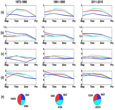
The overall MapReduce processed is shown in Fig. 2 [1, 13]. A client submit a job to the master, which then assign and manage Map and Reduce job parts to slave nodes. Map will read and process blocks of files stored locally in the slave node. The Map output of pair key-values are sent to Reducer.
Blocks in node-1
HDFS
Map
Map
Map
Map
Reduce
Reduce
Reduce
Output1
Output2
Output3
HDFS
Blocks in node-2 Blocks in
node-3
Blocks in node-n
shuffle
Client Hadoop
MapReduce master Job
Job parts
Job parts
Figure 2: MapReduce Processes.
2.4. Parallel k-Means for Hadoop
We have found two parallel k-Means developed for Hadoop environment. The core concept of both is excerpted as follows.
First, in [4], the map function assigns each object to the closest centroid while the reduce function performs the procedure of updating the new centroids. To decrease the cost of network communication, a combiner function combines the intermediate values with the same key within the same map task in a Hadoop node.
The excerpt of the algorithm of Map, Combine and Reduce (detailed algorithm can be found in [4]): (a) Map-function: The input dataset is stored in HDFS as a sequence file of <key, value> pairs, each of which represents a record/instance/object in the dataset. Map computes the minimum distance for each object to all centroids. It then emits strings comprising of the index of its closest centroid (as key’) and object attributes (as value).
(b) Combine-function: Processing key-value pair from Map, Combine partially sums the attribute values of the points assigned to the same cluster and number of objects in each cluster. It emits strings comprising of the index of its cluster centroid (as key’) and the sum of each attribute value of objects in this cluster.
(c) Reduce-function: Reduce function sums all the samples and compute the new centroids (centers)
which are used for next iteration. It then emits key’
is the index of the cluster, value’ comprising a string
representing the new centroids.
Secondly, in [5], the parallel K-means algorithm is improved by removing noise, giving pre-computed value of k and initial clusters (to reduce iterations). The excerpt of the general idea: The value of each attribute for each object is evaluated, then based on this value a GridId is assigned for each object. Object having attribute values beyond its threshold is removed. The centroid of the grids
are fed into DBSCAN algorithm to obtain the best k
value (the k initial cluster centers are computed from
the sample of grids). The k and initial clusters are used as input of Map function of parallel k-Means based on MapReduce.
Some drawbacks that we found on those existing parallel k-Means are:
(a) Big data may (most likely) contains noise or outlier and missing value, hence it must be handled. If cleaning data is performed before the big data is fed into k-Means, it will be inefficient. This has not been addressed in the algorithm.
(b) The Reduce function emits cluster centroids only as patterns. For some big data, such as organizations business data, this may not be sufficient.
(c) If some more patterns need to be computed (in the Reduce) that require detailed information (attribute values) of each object, Combine (that sums up attribute values of “local cluster”) cannot be employed.
(d) In [5], the formula for obtaining GridId is not presented clearly. While an object may have several attributes, the GridID of an object is computed
[image:4.612.200.428.169.342.2]1848 (e) As the parallel DBSCAN algorithm is not included in the proposed technique, it seems that initial centroids are still computed at the outside of Hadoop system.
By examining those drawbacks, we aim to develop a parallel k-Means with the capability to preprocess the big dataset and compute suitable metrics that can be used to evaluate cluster quality as well as patterns.
3.PROPOSEDTECHNIQUE
In this section, we present the analysis of selecting cluster quality metrics, the enhancement of providing metrics and pattern components and the parallel k-Means algorithm based on MapReduce.
Our proposed technique is designed based on the MapReduce concept as depicted in Section 2.3. Hence, the parallel k-Means is not applicable for other than Hadoop distributed environment.
3.1. Selecting Cluster Quality Metrics and Pattern Components
Big data may consist of millions or even billions of objects. Clustering big data will produce clusters where each cluster may have very large number of object members. The following is the feasibility review of using metrics depicted in Subsection 2.2 for measuring the quality of big data clusters:
(a) Number of object members: In each iteration, the number of objects in every clusters are computed (and used to compute the new centroids), so having this metrics is feasible.
(b) Standard deviations of cluster attributes and pooled standard deviations of each cluster: The computation of µ in (xi - µ) (Eq. 3) requires that all
of attribute values in every object in each cluster be stored in the slave node memory. Storing the whole (raw) large number of objects and their attribute values in the slave nodes memory will not guarantee scalability (required for good clustering algorithm) in processing big data. Accessing each object (of million objects) in each iteration also worsens the time complexity. As a solution, we propose the following approach: As in each k-Means iteration the cluster centroids are closer to the final centroids, the cluster centroids obtained
from the previous iteration is used as µ in the
current iteration such that while iterating the list of
values (that include xi), Reducer functions compute
(xi - µ) along with other computations (to produce
pattern components). Then, after all of the
computations are performed, the standard
deviations of each attribute (SDj) and pooled
standard deviation (SD) can also be computed.
(c) Separation of the clusters: Computing silhouette
coefficient of each clustered object, S(i), requires
that the whole (raw) large number of objects and their attribute values be stored in the slave nodes memory in every k-Means iteration. This is
necessary because a(i) and b(i) computations in Eq.
6 need distance computation from one object to every other object in its cluster as well as other clusters. If this metric is adopted for clustering big data, the computation will worsen the scalability and time complexity of the parallel k-Means. Hence, it is not feasible to be adopted.
Based on those analysis, the metrics chosen for evaluating cluster quality are number of members and pooled standard deviations for every cluster.
As discussed in Subsection 2.2, number of members and standard deviation of attributes in clusters can be regarded as cluster pattern components. Hence, we can include these as part of the patterns for reducing computations. Other components that we adopt are cluster centroids, the minimum and maximum of attribute values in every cluster. Computing those 5 pattern components will not add significant time complexity as it can be performed along with clustering process in every iteration.
3.2. Parallel Clustering Technique
In our previous work presented in a conference [7], we proposed a technique for clustering big data consisting of two stages that include data sampling for finding initial centroids and some enhancement as the following:
(1) Data preprocessing: Attributes selection, cleaning and transformations are performed along with the clustering process, in the Map functions that takes input the raw dataset. Hence, the big data is not “visited” more than once.
(2) Reducing iterations: MapReduce known for its inefficiency in iterative processes (such as in k-Means algorithm) as in each pass the output must be written in HDFS. Reducing the iterations number is significant. We propose that initial centroids be computed by MapReduce from a sample of dataset, which are expected to be closer to the final centroids.
(3) Adding computations in Reduce function for computing some pattern components. In this past research, we had not conducted experiments to support our concept.
In [7], we present experiment results showing that the proposed technique is scalable but have not conducted experiments with real big data set for evaluating the cluster patterns.
1849
centroids close to the real ones. Hence, that technique needs to be revised as depicted on Fig. 3.
patterns
2 enhanced
paralel k-Means 1
computing initial centroids
initial centroids
HDFS
HDFSFigure 3: Proposed Clustering Technique.
The technique consist of 2 processes where the detailed design is discussed below.
Process-1:
Determining the initial centroids can be done by clustering a sample of dataset or other technique. The algorithm for parallel sampling and clustering the sample is discussed in [7].
Process-2:
This k-Means performs data preprocessing and produces metrics for measuring clusters quality and pattern components of each cluster at each iteration as follows:
(1) Mapper: Performs
a) Cleaning, attributes selection and
transformations or normalizations;
b) Finding the closest centroid for each object (Eq.
2) and emit ID Cluster as the key and IdObject,
the object distance to its centroid, the attribute values of this object as the value.
(2) Reducer: By receiving key and list of value, Reducer produces metrics of cluster quality as well as pattern components as follows:
a) Compute number of object members in each
cluster, new centroids, sum of the distance of
each object to its centroid (distCluster),
minimum, standard deviation of each attribute value, pooled standard deviation for each cluster, and average SSE (Eq. 5). This computation is performed based on the Section 3.A analysis and approach.
b) Emit and write the IdCluster and all of the
computation results.
(3) Job (main program): (a) Submitting MapReduce
functions to the master node; (b) Computing the cost
function by summing up all of the distCluster value
(of each cluster), Ji (Eq. 1) obtained from Reduce
output; (c) Checking the convergence by examining the value of |Ji – Ji-1|, if it is greater than the
minimum cost then replace the initial centroids with
the current centroids and repeat the iteration by submitting MapReduce functions to the master node. Otherwise, stop the iteration.
The detailed algorithm is presented below.
Algorithm: Enhanced parallel k-Means
This k-Means consists of four algorithms as depicted below (as improvement of the proposed algorithm in [7, 14]).
Algorithm kM-1. configure
Input: Initial centroid file, fInitCentroids
Output: centers[][]
Descriptions: This algorithm is executed once before map is called where it fills the array of
centroids, centers, from initial centroid file,
fInitCentroids.
Algorithm kM-2. map
Input: initial or current centroids, centers[][]; an
offset key; a line comprising object attribute values,
value; a set of valid min-max value for every attribute
Output: <key’, value’> pair, where the key’ is the Id
of the closest centroid and value’ is a string
comprise of object information Steps:
1. Initialize arrRawAtr[] and arrAtr[]
2. Get each of the object attribute valuefrom value,
store in arrRawAtr[],
3. arrAtr[] = results of preprocessing arrRawAtr[], where preprocessing include data cleaning and transformation
1850 determine the object’s cluster based on the
closest centroid
4. construct value’ as a string comprising distance
of the object to its cluster centroid and the values of arrAtr;
5. emit < index, value’>;
Algorithm kM-3. reduce
Input: index of the cluster, key; list of ordered values
from all of hosts, ListVal; array of centroids from
previous iteration, prevcenters;
Output: < key’, value’> pair, where the key’ is the
index of the cluster, value’ is a string comprising:
centers[] (centroid of a clusters), number of objects
in a cluster, countObj, minimum, maximum,
average, standard deviation of every attribute,
pooled standard deviation for a cluster, minAtrVal[],
maxAtrVal[], StdAtrCluster[], PooldStdCluster;
currentCostFunction, J; averageSSE, AvgSSE.
Steps:
1. Initialize minAtrVal[], maxAtrVal[],
SumDiffAtrPrevCenter[], SumAtr[],StdAtrCluster [], centers[]
2. countObj = 0; J = 0;
3. While(ListVal.hasNext())
4. get the object attribute values and its distance
to centroid from value
5. for each attribute, add its value to SumAtr[]
accordingly, subtract its value with its previous
centroid stored in prevcenters, compute the square
of this result then add this to SumDiffAtrPrevCenter
accordingly, compare its value to the corresponding
element value in minAtrVal, maxAtrVal, replace
value in minAtrVal, maxAtrVal,
6. J = J + dist;
7. countObj = countObj + 1
8. Compute new centroids by dividing SumAtr with
countObj and store the results in centers;
10. Compute approximate of standard deviation of every attribute in each cluster using
SumDiffAtrPrevCenter, store the result in StdAtrCluster accordingly
11. Compute PooldStdCluster using StdAtrCluster
based on Eq. 3 and 4
12. Compute AvgSSE by dividing J by countObj
11. Construct value” as a string comprising
countObj, centers, J, minAtrVal, maxAtrVal, StdAtrCluster, PooldStdCluster, AvgSSE 12. Emit < key, value”>;
Algorithm kM-4. run (the Hadoop job)
Input: Array of cost function, J; maximum of
iteration, maxIter; minimum of the different
between current and previous iteration of cost function, Eps.
Output: J
Steps:
1. Initialize J[maxIter]; 2. iter = 1;
3. While iter <= maxIter {execute configure, map
and reduce function; get J from the output of reduce
function then store it in J[iter]; if absolute value of
(J[iter] – J[iter-1]) <= Eps then break; else iter = iter + 1}
4.EXPERIMENTS
We have implemented the algorithms and performed a series of experiments using big dataset in a Hadoop cluster with a master (name node) and 6 slave nodes. All of the nodes are commodity computers having low specification with processor of Quad-Core running at 3.2 GHz clock and RAM of 8 Gb.
Dataset: The dataset of household energy
consumption is obtained from:
https://archive.ics.uci.edu/ml/datasets/ with the size of approximately 132 Mb. This archive contains 2075259 measurements (records) gathered between December 2006 and November 2010 (47 months). The sample of the dataset are as follows:
9/6/2007; 17:31:00 ; 0.486 ; 0.066; 241.810; 2.000; 0.000 ; 0.000 ; 0.000
9/6/2007; 17:32:00 ; 0.484 ; 0.066; 241.220; 2.000; 0.000 ; 0.000; 0.000
9/6/2007; 17:33:00 ; 0.484 ; 0.066 ; 241.510; 2.000; 0.000 ; 0.000 ; 0.000
Each line presents a record with 9 attributes, the excerpts are:
(1) Date; (2) Time;
(3, 4, 5, 6) some results of metrics;
(7) sub_metering_1: energy sub-metering (watt-hour) that corresponds to the kitchen,
(8) sub_metering_2: energy sub-metering that corresponds to the laundry room;
(9) sub_metering_3: energy sub-metering that corresponds to a water-heater and an air-conditioner.
Mining objective: By understanding the dataset, the objective that is feasible is to obtain energy consumption patterns of the household. Knowing this, the power provider may design better services for this household.
1851
a) Number of day (1, 2, …7) is extracted from
Date and stored as attribute-1;
b) Hour (1, 2,…24) is extracted from Time and
stored as attribute-2;
c) The value of sub_metering_1, _2 and _3 are
taken as is and stored as attribute-3, -4, -5. Thus, the preprocessed dataset has 5 attributes, which are day number, hour and 3 sub-metering measures.
Testing the performance of the proposed parallel k-Means: For experimenting speed and scalability, we created several simulation dataset
with the size of 0.2, 0.4, 0.8, …, 2 gigabyte as the “multiplications” of the original dataset. We use HDFS block size of 32 and 64 Mb. We then repeatedly clustered each of the dataset stored using k = 3 for each of the block size setting. We then averaged the execution times on every blocks and plotted the results as depicted on Fig. 5. The speed with 32 and 64 Mb block size is almost the same. The time execution plots are linear, which indicates that the execution of the proposed k-Means scales linearly to the size of dataset or guarantee scalability.
Figure 5: Average Iteration Performances on Two HDFS Block Sizes.
Mining knowledge from the dataset: The
experiments for obtaining the best k, patterns and
knowledge are presented as follows.
Selecting the best k using the cluster quality
metrics: This experiment is intended to show how
to use the proposed quality metrics for finding the
best cluster number, k. We cluster the preprocessed
dataset with k = 3, 4, 5, 6 and 7. The count of iterations until k-Means reach convergence and the
average execution time (in seconds) for each k are:
k = 3: 11 - 60; k = 4: 10 - 61.88; k = 5: 15 - 63.13;
k = 6: 15 - 65 and k = 7: 16 - 66.25. The results for
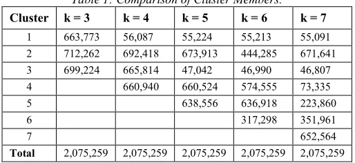
[image:8.612.179.431.261.402.2]each metrics are depicted in Table 1, 2 and 3.
Table 1: Comparison of Cluster Members.
Cluster k = 3 k = 4 k = 5 k = 6 k = 7
1 663,773 56,087 55,224 55,213 55,091
2 712,262 692,418 673,913 444,285 671,641
3 699,224 665,814 47,042 46,990 46,807
4 660,940 660,524 574,555 73,335
5 638,556 636,918 223,860
6 317,298 351,961
7 652,564
[image:8.612.178.435.530.648.2]1852
Table 2: Comparison of Pooled Standard Deviation.
Cls k = 3 k = 4 k = 5 k = 6 k = 7 1 16.20 200.57 174.51 174.47 173.95 2 70.61 35.75 15.37 12.25 14.69 3 132.48 68.75 196.41 196.31 196.01
4 11.53 10.29 8.32 15.39
5 30.42 30.25 19.91
6 9.80 14.87
[image:9.612.310.511.101.230.2]7 8.44
Table 3: Comparison of Average SSE.
Cls k = 3 k = 4 k = 5 k = 6 k = 7 1 3.52 13.21 12.57 12.57 12.55
2 6.06 5.01 4.09 3.28 4.06
3 9.06 7.23 14.01 14.01 13.99
4 3.44 3.42 3.02 4.04
5 5.81 5.79 3.87
6 3.09 3.38
7 3.33
Note: Cls = cluster
Based on the metric results, the best k is selected as
follows:
a) By comparing the number of cluster members
(Table 1), k = 3, 4 and 5 can be selected as the
candidates of the best k as there is no obvious dominating cluster (there are at least 3 clusters that have almost equal members).
b)
Among the clustering results with k = 3, 4 and5, by examining the contents of Table 2 and 3, it is found that for k = 3:
• the maximum of standard deviations
(belongs to cluster 3), which is 132.48, is less than 200.57 (cluster 1 in k = 4) and 174.51 (cluster 1 in k = 5);
• the maximum of average SSE (belongs to
cluster 3), which is 9.06, is less than 13.21
(cluster 1 in k = 4) and 12.57 (cluster 1 in
k = 5).
Hence, it can be concluded that the best k is 3 and
the clustering patterns can be interpreted from the 3 clusters.
Pattern interpretation of 3 clusters: The
components of the patterns, which are the average (centroids) and deviation of each attribute for every cluster and member of each cluster is shown on Fig. 6. The other pattern components, which are the minimum and maximum of the 5 attribute values are as follows:
a) Cluster-1: minimum: 1,0,0,0,0; maximum: 7,
10, 45, 76, 13;
b) Cluster-2: minimum: 1, 7, 0, 0, 0; maximum: 7,
23, 81, 80, 11;
c) Cluster-3: minimum: 1,0, 0, 0, 4; maximum: 7,
23, 88, 78, 31.
Figure 6: Patterns of Three Clusters (Cluster-1 = pink, 2 = green, 3 = blue).
As attribute 1, 2, 3, 4, and 5 corresponds to number of day, hour, results of energy submeter in the kitchen, laundry room, and water-heater and air-conditioner, the interpretations of the pattern for each cluster are as follows:
a) Cluster-1 (pink): As the centroids of
submeter-1,-2,-3 value are low while standard deviations are also low with almost one-third of the members, this means that most of the day at the early of hour, in the whole house (on 3 sub-meters), the energy consumption are low. Sometimes the house do not use electricity at
all and the maximum energy usage in 3 submeters are 45, 76 and 13.
b) Cluster-2 (green): The centroids of the hour is
[image:9.612.103.507.465.541.2]1853
c)
Cluster-3 (blue): The centroids of the hour israther high, submeter -1,-2 (kitchen and laundry) values are low, submeter-3 value is high, while standard deviations of the hour, submeter-1 in the kitchen is high (with maximum value of 88) and submeter-2 in the laundry room are quite high (maximum value is 78), and submeter-3 is low, with almost one-third of the members. This means that most of the day at around mid-day, the average energy consumption in the kitchen and laundry are low but with high fluctuation, while water-heater
and an air-conditioner is almost always high.
Based on the patterns interpretation of those 3 clusters, the overall knowledge can be summarized as follows: The family consume low energy at most of the time. But, they frequently use water-heater and air condition during mid-day and sometimes do laundry during also around the mid-day. This knowledge seems to be logical or make sense. Hence, this experiments prove that the 3 quality cluster metrics and 5 components of cluster pattern can be adopted for clustering big data.
To show that the pattern components are also useful for clustering other big data, in the Appendix A, we present the experiment results for mining historical weather patterns from big data recorded by weather stations.
5.CONCLUSION
Parallel k-Means based on MapReduce can further be enhanced by adding the capability for computing metrics that can be used for evaluating cluster quality as well as generating patterns from big data. The computations are included in the Reduce function. Our experiment results using big datasets show that time execution scale linearly and the metrics are useful for finding knowledge. However, we have not address the metrics for measuring separation of the clusters. Hence, this issue is left for further works.
For finding the best k using our proposed
technique, big data is clustered several times. Also, in every iteration of k-Means, big data is read from HDFS. Both of these lead to inefficiency. Hence, further improvement of the proposed technique is required. One option for reducing the number of reading HDFS is by storing the big data in parallel
memory. While for finding the best k, other
technique may be employed. One option is by enhancing grid-based clustering technique in the parallel computation environment.
ACKNOWLEDGMENT
We like to thank to the Directorate General of Higher Education of Ministry of Research, Technology and Higher Education of the Republic of Indonesia who is funding this research in 2016-2017 through Hibah Bersaing scheme with contract number of III/LPPM/2016-06/134-P.
REFERENCES
[1] A. Holmes, 2012. Hadoop in Practice, Manning Publications Co., USA.
[2] J. Han and M. Kamber, 2011. Data Mining
Concepts and Techniques 2nd Ed., Morgan
Kaufmann Pub., USA.
[3] K. Tsiptsis and A. Chorianopoulos, 2009. Data Mining Techniques in CRM: Inside Customer Segmentation, John Wiley and Sons, L., UK. [4] W. Zhao, H. Ma and Q. He, 2009. “Parallel
K-Means Clustering Based on MapReduce”, CloudCom 2009, LNCS 5931, pp. 674–679, Berlin Heidelberg: Springer-Verlag.
[5] L. Ma, L. Gu, B. Li, Y. Ma and J. Wang, 2015. “An Improved K-means Algorithm based on
Mapreduce and Grid”, International Journal of
Grid Distribution Computing, vol.8, no.1, pp.189-200.
[6] Berry, M.J.A. and Linoff, G.S., 2004. Data Mining Techniques for Marketing, Sales and
Customer Relationship Management, 2nd Ed,
Wiley Publ., USA.
[7] V. S. Moertini and L. Venica, 2016. Enhancing Parallel k-Means Using Map Reduce for Discovering Knowledge from Big Data, Proceedings of the 2016 Intl. Conf. on Cloud Computing and Big Data Analysis (ICCCBDA 2016), pp. 81- 87, Chengdu China, 5-7 July. [8] Jang, J.-S.R.; Sun, C. –T and Mizutani E., 1997.
Neuro-Fuzzy and Soft Computing, Prentice Hall Inc., USA.
[9] Moertini, V.S., 2002. “Introduction to Five Data
Clustering Algorithms”, Integral, Vol. 7, No. 2,
pp. 87-96.
[10] S. Chius and D. Tavella, 2011. Data Mining and Market Intelligent for Optimal Marketing
Returns, Routledge Pub., UK.
[11] S. Padmaja and A. Sheshasaayee, “Clustering of User Behaviour based on Web Log Data using Improved K-Means Clustering
Algorithm”, International Journal of
Engineering and Technology (IJET), Vol. 8, No 1, pp. 305-310, 2016.
1854 [13] E. Sammer, 2012. Hadoop Operations,
O’Reilly Media, Inc., USA.
1855 APPENDIX A
MINING HISTORICAL PATTERNS FROM WEATHER DATA
This experiment is intended to show the use of the proposed technique for obtaining patterns and knowledge from the big historical data of weather.
Dataset:The data is downloaded from NOAA's National Centers for Environmental Information, http://www1.ncdc.noaa.gov/pub/data/noaa/. There are thousands of files which are stored and organized based on the measurement year (1901, 1902, ….2015, 2016). Each file represent measure results from a station in a single year and named using the format of XXXXXX-NNNNN-YYYY.gz (for example, 010010-99999-1973.gz and 072010-99999-1991.gz) where XXXXXX represents the station number, NNNNN is WBAN weather station identifier and YYYY denotes year. The size of each file varies, depending on the frequency of measurements. Total size of all files are more that 500 Gb. Each file contains records of weather measures for a station in a year. Each record is presented in one line and represented in text string and consists of 31 attributes, such as station identifier, observation date, time, latitude, longitude of observation point, elevation, wind direction, wind speed, visibility distance, air temperature, dew point temperature, atmospheric pressure and other attributes. One example of file content (one records) are as follows:
0207010010999992001010118004+70930-008660FM-12+0009ENJA V0203501N004610090019N0200001N1-
00711-00901100351ADDAA112000791AY181061AY231061
GF108991071081004501041999KA1120M-00401MA1999999100231MD1110041+9999MW1031R EMSYN094AAXX 01184 01001 11470 83509 11071 21090 30023 40035 51004 69902 70383 8784/ 333 11040 91114;
The objectives: Mining patterns of “snapshots” of the historical data weather and then comparing the resulted patterns of each snapshot for observing weather changes across the periods. In these experiments, the patterns are produced from the four selected attributes, which are wind speed,
temperature, dew point temperature and
atmospheric pressure.
Data selection and preprocessing: In order to observe meaningful weather pattern changes, it would be improper if the whole weather data are analyzed at once as the data are measured from all over places/points of the world at various altitude and longitude having 4 seasons (summer, fall, winter and spring) or tropical seasons (simply rainy and dry). Instead, weather data should be selected from a station or some nearby stations. Aiming to obtain historical patterns, we cluster the data from consecutive “snapshot” periods. Some example of the periods are 1973-1980, 1981-1985, 1986-1990, 1991-1995, …., 2010-2015. We then cluster the data at each snapshot time using the four selected attributes, analyze and compare the patterns generated.
Data selection and preprocessing in Map functions:
a) As Map function can take HDFS folder name
containing those thousands of files and the data weather is presented in files having their station number and year measured, we define the station numbers as well as the snapshot periods as Map variables such that Map select and read the files associated with the stations and the snapshots time at each pass.
b) Map then select the 4 attributes and transform
these as follows: (1) Wind speed, temperature, dew point temperature are divided by 10 (as the recorded data are multiplied by 10, we normalized those into their real values); (2) Pressure is divided by 1000 such that this attribute value does not differ greatly with the others, which could lead into the most dominant attribute (in calculating the object distance using Euclidean method).
Defining k and clustering process: We have clustered the snapshots of weather data from few stations. Here, we present the experiment results of clustering the 8 snapshot data from station 010010 at Jan Mayen (Nor-Navy) Norway as an example. Expecting to obtain patterns related to cold, middle and hot seasons, we cluster the data of each of the 8 snapshots (1973-1980, 1981-1985, 1986-1990,
1991-1995, …., 2010-2015) into 3 clusters (k = 3).
The number of k-Means iterations (until
1856
Table A.1: Iterations and execution times of data from a station at Norway
Period #Iterations Time (sec) AvgTime (sec)
1973 - 1980 11 426 39
1981-1985 22 872 40
1986-1990 9 349 39
1991-1995 13 512 39
1996-2000 9 354 39
2001-2005 17 676 40
2006-2010 15 581 39
2011-2015 15 603 40
Average 13.875 546.64 39.32
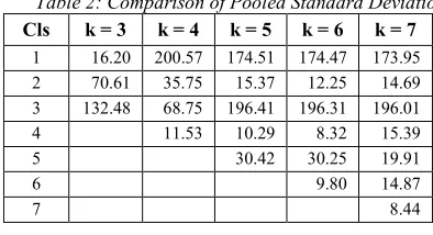
Interpreting patterns: In Fig. A.1, we present the sample of patterns obtained from 3 snapshot periods (1973-1980, 1991-1995 and 2010-2015) only. Each cluster pattern is represented with blue, magenta and red plots. The pattern components are centroids, deviations, minimum, maximum of
attribute values in each cluster and object members.
Wsp: wind speed, Tem: air temperature, Dew: dew point temperature, Prs: atmospheric pressure.
[image:13.612.119.496.305.664.2]1857 Some observable of weather changes interpreted from the patterns as follows:
a) Centroids: While the magenta and read seem to
be steady, the blue cluster dew point temperatures increased starting from 1991-1995 snapshot.
b) Deviations: The wind speed differ greatly in
blue cluster, the attribute values of the blue one differ the most (have the most variety values), while the pressure differ slightly only at all clusters.
c) Minimum attribute values: the blue cluster dew
point temperatures also increased starting from 1991-1995 snapshot.
d) Maximum attribute values: no obvious change
found.
e) Cluster member: If the weather data were
recorded evenly from this station during those snapshot, the following is the interpretation: (1) In 1973-1980, Jan Mayen was mostly
warm/hot; (2) In 1973-1980 and 2011-2015,
the blue cluster (cold weather) have smaller members; (3) In 1991-1995, the members number of blue and red cluster differ slightly suggesting that the cold weather happened almost as long as hot weather.
![Fig. 2 [1, 13]. A client submit a job to the master, The overall MapReduce processed is shown in parts to slave nodes](https://thumb-us.123doks.com/thumbv2/123dok_us/8907217.957381/4.612.200.428.169.342/client-submit-master-overall-mapreduce-processed-shown-parts.webp)