www.nat-hazards-earth-syst-sci.net/9/1897/2009/ © Author(s) 2009. This work is distributed under the Creative Commons Attribution 3.0 License.
and Earth
System Sciences
A GIS-based numerical model for simulating the kinematics of mud
and debris flows over complex terrain
S. Beguer´ıa1, Th. W. J. Van Asch2, J.-P. Malet3, and S. Gr¨ondahl3
1Aula Dei Experimental Station, Spanish National Research Council (CSIC), Zaragoza, Spain 2Department of Physical Geography, University of Utrecht, Utrecht, The Netherlands
3Institut de Physique du Globe de Strasbourg, School and Observatory of Earth Sciences (EOST), Strasbourg University, Strasbourg, France
Received: 16 February 2009 – Revised: 20 July 2009 – Accepted: 4 November 2009 – Published: 17 November 2009
Abstract. This article presents MassMov2D, a two-dimensional model of mud and debris flow dynamics over complex topography, based on a numerical integration of the depth-averaged motion equations using a shallow water ap-proximation. The core part of the model was implemented using the GIS scripting language PCRaster. This environ-ment provides visualization of the results through map ani-mations and time series, and a user-friendly interface. The constitutive equations and the numerical solution adopted in MassMov2D are presented in this article. The model was ap-plied to two field case studies of mud flows on torrential allu-vial fans, one in the Austrian Tyrol (Wartschenbach torrent) and the other in the French Alps (Faucon torrent). Existing data on the debris flow volume, input discharge and deposits were used to back-analyze those events and estimate the val-ues of the leading parameters. The results were compared with modeling codes used by other authors for the same case studies. The results obtained with MassMov2D matched well with the observed debris flow deposits, and are in agreement with those obtained using alternative codes.
1 Introduction
Mud and debris flows can be defined as gravity-driven flows of a highly saturated mixture of debris in a steep channel, which exhibit properties of viscous and turbulent flows. Ac-cording to Hungr et al. (2001), the difference between debris and mud flows is related to the significantly greater water content of the latter, which causes a plastic behavior (plastic-ity index higher than 5%). Mud and debris flows can
origi-Correspondence to: S. Beguer´ıa
nate either at a single source, typically from the fluidization of a failed mass (landslide), and/or by the re-entrainment of sediment accumulated in a torrential catchment. Fluidiza-tion of the mass usually requires a large amount of water, but rather dry clastic avalanches can also show flow-like be-havior due to grain collisions, and flow on surfaces less in-clined than the angle of repose of the material. When debris flows are confined on a torrent, they can propagate over very large distances before final spreading over an alluvial fan. Debris flows are a common and important factor in erosion and sediment transfer in mountainous areas, and constitute an important risk to the population. The threats to human life and property from mud and debris flows are greater than those of some other landslide types, due to their higher veloc-ity (sometimes in the order of tens of m s−1) and capacity to propagate even on very gentle slopes (below 5◦). Issues
iden-tified in recent reviews of the physics of debris flows include the phenomenon of dilatancy; the roles of grain collisions, internal friction and cohesion; the mechanisms of fluidiza-tion; and the phenomena of particle segregation and depo-sition (e.g. Iverson and Denlinger, 1987; Takahashi, 1991; Hutter et al., 1996; Iverson, 1997).
have been developed for both one-dimensional (Hungr, 1995; Fraccarollo and Papa, 2000; Arattano and Franzi, 2003; Naef et al., 2006) and two-dimensional cases (Savage and Hutter, 1989; O’Brien et al., 1993; Shieh et al., 1996; Laigle and Coussot, 1997; Chen and Lee, 2000; Iverson and Denlinger, 2001; Pudasaini et al., 2005; Hungr and McDougall, 2008). Two-dimensional (2-D) models are becoming common tools for the analysis and prediction of mass movements includ-ing rock avalanches, earth and debris flows, and mud flows. On 11–12 December 2007, a benchmarking exercise on land-slide runout modeling was organized in Hong Kong as part of the 2007 International Forum on Landslide Disaster Man-agement, comparing various 2-D codes (Ho and Li, 2007).
The main objective of this article is to describe the de-velopment and implementation of a numerical code, Mass-Mov2D (a copy of which can be downloaded from http: //hdl.handle.net/10261/11804), for simulating mud and de-bris flows over complex topography, implemented in the PCRaster GIS environment (Wesseling et al., 1996; Karssen-berg et al., 2001). The model is based on a 2-D finite differ-ence solution of a depth-averaged form of the fluid dynamics equations. The flow is thus treated as a one-phase material, whose behavior is controlled by rheology (i.e. by a functional relationship between strain and stress). Several flow laws can be implemented within a common numerical scheme in the model, which can accept a detailed description of a complex topography through a digital elevation model (DEM), thus facilitating simulation of field case studies.
In contrast to other codes, the purpose of the model de-scribed here is to serve as a generic framework within which various modeling concepts can be tested. The model is flex-ible enough to work with various configurations of the ini-tial and boundary conditions, a characteristic that will allow researchers to adapt the simulation to a variety of realistic situations, ranging from alluvial fan dispersion to channel overflow problems. The implementation of several rheolog-ical models allows comparison of various flow types. The model was implemented in a geographical information sys-tem (GIS) package, thus benefiting from a set of tools that fa-cilitate the preparation of input data and evaluation of the re-sults. However, implementation in a GIS platform is benefi-cial beyond being the mere pre- and post-preprocessing tools available, as the core equations of the model (mass balance, equation of motion, rheology) are accessible to the user in an easy-to-learn scripting language. This enables easy testing of new modeling concepts through modification of the original code.
We first describe the governing equations of the model, the various flow laws, the numerical implementation and the specification of the initial and boundary conditions, and pro-vide examples of the model operation. We then present a case study showing the results of application of the model to two debris flow events on torrential alluvial fans, one in the Austrian Tyrol (Wartschenbach torrent) and the other in the French Alps (Faucon torrent).
2 Model description
2.1 Governing equations
The approach was based on the classical Savage-Hutter the-ory (Savage and Hutter, 1989), which assumes a one-phase homogeneous material with rheological properties. The flow was modeled as a 2-D continuum medium using a depth-integrated approximation of the flow dynamics equations; this has become a classical approach to debris flow modeling (Savage and Hutter, 1989; Laigle and Coussot, 1997; Frac-carollo and Papa, 2000; Denlinger and Iverson, 2001; Mc-Dougall and Hungr, 2004; Mangeney-Castelnau et al., 2005; Pirulli et al., 2007). Depth integration is based on the shal-low water assumption (Saint Venant equations), which ap-plies where the horizontal length scale (length of the flowing mass) is much greater than the vertical length scale (thick-ness of the flowing mass). In these conditions the vertical velocity of the fluid is small, so that the vertical pressure gra-dient is nearly hydrostatic. Integration over the flow depth allows a 2-D description of the flow, avoiding the much more complex 3-D formulations. There is experimental evidence of agreement with the experimental data (Savage and Hutter, 1989; Greve and Hutter, 1993).
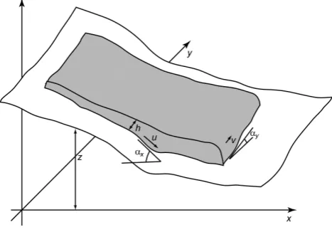
Contrary to depth-integrated models that use a local refer-ence frame linked to the topography, the equations governing MassMov2D are referenced in a 2-D Euclidean space with Cartesian coordinatesx,y (Fig. 1). Very similar formula-tions have recently been proposed (Mangeney et al., 2007). The mass (1) and momentum (2) balance equations were de-veloped as:
∂h ∂t +cx
∂ (hu) ∂x +cy
∂ (hv)
∂y =0, (1)
∂u ∂t +cxu
∂u ∂x+cyv
∂u
∂y = −cxg
Sx+k∂(c∂xxh)+Sfqx
∂v ∂t +cyv
∂v ∂x+cxu
∂v
∂y = −cyg
Sy+k∂(∂ycyh)+Sfqy
, (2)
respectively, whereh is the flow thickness in the direction normal to the bed (L); (u,v) are the x and y components of the velocity vector along the bed (L T−1); the coefficients cx=cosαxandcy=cosαyare the direction cosine of the bed
(geometry factors to correct from local to global reference systems); andαxandαyare the values of the angle between
Fig. 1. Reference frame used in MassMov2D.
Sx=tanαxandSy=tanαyare the bed slope gradient in thex
andydirections (L L−1), respectively. The spatial derivative in the second term is the pressure acceleration, i.e. the time rate of change due to pressure differences within the flow. Sf is the flow resistance gradient (L L−1), which accounts
for momentum dissipation within the flow due to frictional stress with the bed (see next section).
The term k in Eq. (2) is the earth pressure coefficient, i.e. the ratio between the tangential and normal stresses. It has a value of 1 for a perfect fluid, but can vary greatly for plastic materials (Savage and Hutter, 1989; Hungr, 1995), and ranges between two extreme values corresponding to the active and passive states in the Rankine theory, i.e.ka≤1≤kp.
These values depend on the internal friction angle of the mix-ture,δ:
ka = 11−+sinsinδδ
kp= 11+−sinsinδδ
(3)
The active statekaapplies to regions of the flow that undergo
expansion,
cx
∂ (uh) ∂x +cy
∂ (vh) ∂y ≥0.
The passive state kp corresponds to regions experiencing
compression,
cx
∂ (uh)
∂x +cy ∂ (vh)
∂y <0.
Finally,qxandqyare coefficients:
qx =√−u u2+v2 qy =√−v
u2+v2
, (4)
where the minus sign beforeuandvensures thatSf opposes
the direction of the velocity.
2.2 Flow laws
The flow termSf in Eq. (2) represents the bed shear stress
of the flow, which is responsible for energy dissipation. This variable describes the rheological properties of the flow, which control flow behavior. The model defined by Eqs. (1) and (2) is therefore valid for different types of flows, depend-ing on the formulation ofSf. One-phase, depth-integrated
models characterize flow behavior by a rheological relation-ship, and typically assume homogeneous and constant flow properties. These simplified models are preferred for applied field studies because of their parsimony, which makes them more suitable for calibration and back-analysis. A number of rheological models for the flow term have been reviewed by Naef et al. (2006).
Mud and debris flows have often been modeled as vis-coplastic materials with a laminar flow regime, i.e. as Bing-ham fluids with constant yield strength and viscosity (Cous-sot, 1994). A linear stress-strain rate relationship is assumed once the yield strength is exceeded. However, a convex re-lationship defining a shear thinning behavior (i.e. decreasing viscosity with applied shear) is in better agreement with most experiments, and led to definition of the Herschel-Bulkley model. Both models can be described by the following rela-tionship:
τ (z)=τC+µ ∂v
∂z β
, (5)
whereτ (z) is the resisting shear stress at a given depth z (M L−1T−2),τCis a constant yield strength due to cohesion,
∂v/∂zis the shear rate, andµ (M L−1T−1)-beta is a con-sistency index acting as a viscosity parameter. The viscos-ity of the flow is closely related to the percent concentration of solids (O’Brien and Julien, 1988; Parsons et al., 2002), and can range from 10−2to 103. The exponentβ is an em-pirical parameter of value 1 in the Bingham model, and in the Herschel-Bulkley model has to be determined with the aid of experimental data. A number of debris flow models are based on rheological formulations for a Bingham viscous fluid, or the Herschel-Bulkley model with different values ofβ (O’Brien et al., 1993; Coussot, 1994; Han and Wang, 1996; Laigle, 1997; Laigle and Coussot, 1997; Fraccarollo and Papa, 2000; Zanuttigh and Lamberti, 2004; Remaˆıtre et al., 2005).
The Bingham/Herschel-Bulkley model is valid for materi-als where the fine fraction is large enough to lubricate con-tacts between grains, i.e. approximately 10% clays size frac-tion (Ancey, 2001; Rickenmann et al., 2006). A more general alternative model is obtained if the constant yield strength in Eq. (5) is replaced by a combined cohesive-frictional com-ponent, leading to the Coulomb-viscous model (Johnson and Rodine, 1984):
τ (z)=τC+(σ−u)tanϕ+µ ∂v
∂z β
, (6)
bed normal stressσ=ρgh(M L−1T−2), whereρ is the ma-terial density (M L−3), u (M L−1T−2) is the internal pore fluid pressure, and ϕ (◦) is the basal friction angle of the
flow. The internal pore fluid pressure is a transient property that is coupled to the normal stress and can dissipate dur-ing motion, makdur-ing it extremely difficult to model. Thus, in most practical applications the pore pressure ratio (u/σ) is assumed to be constant, and hence the frictional dissipation can be lumped into a single parameter (tanϕ0), whereϕ0 is an apparent friction angle. This approach was implemented in MassMov2D, based on the hypothesis that the pore pres-sure is conserved and remains constant during the simulation. Mixed frictional-viscous models similar to that in Eq. (6) are suited to describing the shear behavior of granular solid ma-terials (Naef et al., 2006). The Coulomb frictional-viscous model has also been used to model debris flows (O’Brien et al., 1993; Coussot, 1994; Han and Wang, 1996; Laigle, 1997; Laigle and Coussot, 1997; Fraccarollo and Papa, 2000; Zanuttigh and Lamberti, 2004; Van Asch et al., 2007) and has also been applied to very large landslides in which the forma-tion of a melted rock layer adds extra lubricaforma-tion to the flow (De Blasio and Elverhøi, 2008).
In applying Eqs. (5) and (6) there is a need to integrate the stress over the flow depth, to enable computation of the total stress,Sf. In depth-integrated models this is solved by
assuming that the stress distribution in the direction normal to the flow is triangular. Following Coussot (1997), we have used a simplified form of the third-order Bingham expression for the shear stress to deriveSf:
Sf=
τ0 σ =
1 σ
3 2τC+
3µ h |u|
. (7)
Equation (7) is a good approximation to the original formu-lation for values of the stress ratio (τC/τ) smaller than 0.5
(Naef et al., 2006). For the Coulomb-viscous rheology we have used:
Sf=tanϕ0+
1 σ
3 2τC+
3µ h |u|
. (8)
Hence, for particular simulations the rheology of the flow is defined by a parameter vector(ρ,τC,µ)or ρ,ϕ0,τC,µ
for the Bingham and the Coulomb-viscous laws, respectively. 2.3 Numerical implementation
The numerical implementation of hyperbolic partial differen-tial equations, such as Eqs. (1) and (2) is a challenging task, especially for systems exhibiting an advancing front (see the review by McDougall, 2006). We adopted a reasonably sim-ple compromise solution that achieved a desired level of sta-bility, accuracy and controlled diffusivity.
It is convenient to write Eqs. (1) and (2) in more compact vector notation, in order to describe the numerical solution used in MassMov2D:
∂ ∂tw+k1
∂ ∂xf+k2
∂
∂yg+k3(q+s)=0, (9)
where w= h u v
,f = hu u v
,g= hv u v
,k1 =
cx
cxu
cyv
,
k2=
cy
cyv
cxu
,k3= 0 cx cy
,q=
0 k∂(gcxh)
∂x +g Sx
k∂(gc∂yyh)+g Sy , and s= 0 qxSf
qySf
.
The model was implemented in an explicit finite difference (Eulerian) mesh, i.e. the flow was described by variation in the conservative variables at points of fixed coordinates (i, j) as a function of time (n). The mesh is defined as a regular grid with sizes=1x=1y, in accordance with the grid for-mat common to most GIS platforms. Equation (9) is solved numerically using a central difference forward scheme:
wni,j+1=Wwni,j−1tk1ni,j
fni+1,j−fni−1,j+
k2ni,j
gn
i,j+1−gni,j−1
+k3ni,j
qn i,j+s
n+1/2
i,j
, (10)
where1tis the time step duration (s), and the pressure gradi-ent term in q is computed by cgradi-entral differences. A common problem with such simple methods is the introduction of dis-persive effects that lead to unphysical oscillations, especially in the presence of large gradients. A solution to this problem is the addition of a certain amount of numerical regulariza-tion, as introduced in Eq. (10) by the functionW
wni,j:
Wwni,j=
(1−CFL)wni,j+CFLw n
i−1,j+wni+1,j+wni,j−1+wni,j+1
4 ,
(11)
This function performs a weighted spatial averaging overw, and the amount of numerical regularization is controlled by the value of the Courant-Levy-Friedrichs condition (CFL; see Eq. 12, below) at each point, so it is applied with pref-erence to the areas of the flow that are experiencing sudden changes and have values of CFL typically in the range 0.5– 1. This solution proved to provide only the required amount of regularization needed to avoid numerical instability, while adding just a minimum amount of artificial dispersion. Re-flecting boundary conditions are applied to Eqs. (10) and (11), so if any ofwni−1,j,wni+1,j,wni,j−1 orwni,j+1lie out-side the boundaries of the flow, then they take the value of
wni+1,j,wni−1,j,wni,j+1orwni,j−1, respectively.
deal with this problem a two-step solution was adopted. Hence, the source termsni,j+1/2in Eq. (10) was evaluated at interleaved time steps to reduce over- and undershoots. The velocity components ofwwere estimated at timesn+1/2 by applying Eq. (10) townwith1t=1t /2.
The resulting solution is thus similar to the Lax-Wendroff second-order scheme (Press et al., 2002). To maintain the stability of the solution throughout the simulation, the Courant-Friedrichs-Levy condition CFL<1 must be satis-fied. CFL was calculated at each point of the mesh as: CFL=1t
s
√
2(u) , (12)
The time step duration1t was adapted at each iteration to the highest velocities found in the spatial domain, to ensure that the Courant-Friedrichs-Levy condition was met over the whole computation domain. Despite this variable internal time step, reporting is made at a regular time interval set by the user.
An underlying assumption of the finite difference solution is that of continuity and smoothness of the spatial domain. Although this generally holds true, in some cases the basal topography presents horizontal discontinuities or singulari-ties such as channels (artificial or natural), which are very relevant to the correct simulation of the flow. Such struc-tures can not be adequately represented in a finite differences mesh, as the central difference scheme requires a continu-ous surface. Specification of topographical discontinuities was incorporated into the model such that they are treated as no-flow boundaries unless the flow thickness becomes larger than the difference in height at both sides of the discontinuity. Whenever this occurs, flow is automatically allowed between the two sides of the topographical discontinuity by applying Eq. (10) to the fraction ofh that exceeds the height of the obstacle.
The model was implemented in the PCRaster environmen-tal modeling language (Wesseling et al., 1996; Karssenberg et al., 2001). PCRaster is a scripting language; hence the computation time involved is greater than it would be using a compiled language such as C or Fortran. For this reason the basic vector operators (gradient, divergence) and some func-tions that are used repeatedly in the code, including theW() function in Eq. (10) and other parts of the numerical scheme, were programmed in C and compiled as new PCRaster func-tions. However, the core functions of the model were imple-mented in the PCRaster scripting language, promoting easy understanding and modification of the original code. This makes MassMov2D a convenient tool for researchers inter-ested in testing new modeling concepts.
2.4 Initial and boundary conditions
The model requires three input files comprising the topogra-phy of the bed, and the locations of the inlet and outlet cells. The topography of the bed is a basic input to the model and
is provided in the form of a DEM. The DEM defines not only the basal boundary of the flow, but also the spatial computa-tion domain and the mesh size. No flow is allowed outside the spatial limits of the DEM (closed boundary) except at two specific areas: i) the inlet, a set of contiguous cells where in-put flow is allowed at a rate specified by the user (see below); and ii) the outlet, a set of cells where flow is allowed to exit the computation domain (open boundary). Additionally, a map with the location of topographical discontinuities, such as channels or dikes, can also be set. This map identifies the domain cells that lie inside the channel, as well as the height of the discontinuity in the direction normal to the basal sur-face (m). These files can easily be created as raster maps using standard PCRaster commands.
In addition to these maps, the model requires specification of the input discharge at the cells defined in the inlet map during the simulation time,wtinlt(boundary condition). This can be set either as a constant inflow rate for a specified time interval, or as a transient flow by creating a text file contain-ing three columns that indicate the time variation of the state variables (h,u,v) at the inlet.
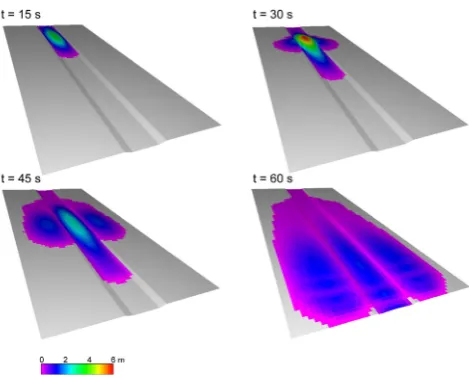
An example of the configuration of a simulation is pro-vided in Fig. 2. A rectilinear channel 150 m long and 3 m deep with a constant gradient α=10.5◦ was defined. The channel borders were treated as spatial discontinuities, mean-ing that only in the case of the flow depth in the channel ex-ceeding 3 m would there be overflow and connection with the flow on the banks. The lateral limits of the spatial do-main were defined as impermeable boundaries, and inlet and outlet boundaries were defined at the upper (upstream) and the lower (downstream) limits. An input discharge file was defined with a triangular shape, rising fromh=0.65 m at 0 s toh=0.85 m at 25 s, and then falling toh=0 m at 30 s. Bing-ham rheology was used, with parameters: ρ=1800 kg m−3, ϕ0=5.5◦ andµ=50 Pa s. Deceleration of the flow along the channel generated an increase of the input wave, and resulted in overflow a few seconds after the peak discharge. After that moment the flow over the lateral banks remained dis-connected from the flow in the channel.
3 Case studies
Fig. 2. Propagation of a mud flow slurry on a rectilinear channel,
causing overflow on the lateral banks. Color scale: flow depth (m).
from the final deposit, which only includes the solid part of the debris flow mixture, requiring that the liquid part be esti-mated.
The simulation of observed events is not only a procedure for validating models, but can also deliver results relevant to case studies. For example, there are no ways to measure directly the rheological properties of the flow, so these need to be calculated by back-analysis using simulation tools.
We used MassMov2D to simulate field events of mud and debris flows in torrential alluvial fans, one in Austria and the other in France. In both cases the simulations were per-formed using the Bingham and Coulomb-viscous rheologies, and the most appropriate values of the rheological parame-ters for each case were established using a heuristic process, comparing the outcomes from different parameter sets with the field deposition patterns. These two events were selected because both had previously been analyzed using other, well-established codes, thus enabling comparison of these results with those from MassMov2D.
3.1 The event of 16 August 1997 in the Wartschenbach torrent
The Wartschenbach torrent is located near Lienz, eastern Ty-rol, Austria. It is a small mountain torrent with a catch-ment area of 2.5 km2 and an altitude ranging from 600 to 2500 m a.s.l. At the bottom the torrent forms an alluvial fan with a mean gradient of 16% (around 9◦). A debris flow
event occurred in the Wartschenbach torrent on 16 August 1997 after an intense storm. A large amount of sediment was trapped in an upstream debris retention dam. Between 25 000 and 30 000 m3of debris and water reached the fan apex. This caused overflow of the little channel, and spread of the de-bris flow over the fan affected 15 buildings (H¨ubl and Stein-wendtner, 2000). The same debris flow event was modeled
by Rickenmann et al. (2006), who compared the results of three different codes for debris flow simulation: DFEM-2D (Naef et al., 2006), FLO-2D (O’Brien et al., 1993) and HB (Laigle, 1997; Laigle and Coussot, 1997).
A pre-event DEM with a grid resolution of 2 m was used in the simulation. The inlet area was located at the fan apex, in the upper part of the DEM. The density of the flow was fixed atρ=2000 kg m−3. In the absence of accurate infor-mation about the input discharge we used a triangular shape with a total duration of 3240 s (54 min) and a total volume of 23 576 m3. Discharge increased from 0 to 15.86 m3s−1at t=1080 s; it remained at this value until t=1440 s and then decreased progressively until t=3240 s. The total simula-tion time was extended untilt=4000 s to allow for the flow to stop. These conditions mimic those used by Rickenmann et al. (2006), so the results of the different models could be compared.
Two simulation experiments were undertaken, using Bing-ham and Coulomb-viscous rheologies. A set of parameter values varying within a reasonable range were chosen, and successive model runs were performed. The results were compared with the field extension and thickness of the de-posit in order to find the best set of parameters. For the Bing-ham rheology the best parameter set wasτC=2500 Pa and
µ=525 Pa s. These results are close to those of Rickenmann et al. (2006), who used the Herschel-Bulkley rheology and found that the best results were obtained with a yield stress value within the range 0.8<τC/ρ<1.35. In our simulation
the value of this ratio was 1.25. Rickenmann et al. (2006) kept the µ/τC ratio constant at 1/3, following Coussot et
al. (1998). We found that the optimum value for this ra-tio was slightly lower, at approximately 1/5. In the case of the Coulomb-viscous rheology, the best parameter set was τC=2500 Pa,µ=1300 Pa s andϕ0=4.8◦.
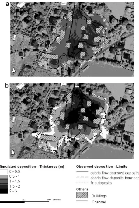
Fig. 3. Simulation of the debris flow event of August 1997 in the
Wartschenbach torrent, using Bingham (a) and Coulomb-viscous
(b) rheologies. Simulation parameters were: τC=2500 Pa and µ=525 Pa s; and τC=2500 Pa, µ=1300 Pa s and ϕ0=4.8◦,
respec-tively.
In addition to the final deposition, map sequences of the flow thickness and velocity at different times (Fig. 4) were produced. The event was characterized by relatively slow velocity, which coincided with eyewitness reports and helped reduce the damage caused by the overflow.
The simulation proved to be more sensitive to changes in τC and ϕ0 than to µ. As found by Rickenmann et
al. (2006), it was difficult to make an independent calibra-tion of the model, as the final results were relatively insen-sitive to small variations in the parameters and because of interactions among the effects of the parameters. For exam-ple, results close to the optimum were obtained using Mass-Mov2D with τC=2200 Pa andµ=550 Pa s for the Bingham
rheology, and with τC=2500 Pa, µ=1400 Pa s, and ϕ0=5.0◦
for the Coulomb-viscous rheology.
3.2 The event of 5 August 2003 in the Faucon torrent
The Faucon torrent is located on the south-facing slope of the Barcelonnette Basin. It has a catchment area of 8 km2 and an altitude ranging from 1170 to 2982 m a.s.l. At the bottom the torrent forms an alluvial fan with a slope of 0.12– 0.08% (5–7◦). The main outcrops are very finely laminated Jurassic black marls, which are mostly covered by moraines and/or slope deposits. The land cover is mainly forest (60%), abandoned agricultural lands, and bare lands with intense gullying. The Barcelonnette Basin has a dry and mountain-ous Mediterranean climate with strong inter-annual rainfall variability (733±412 mm over the period 1928–2002), strong storm intensities (over 50 mm h−1), and more than 100 days of freezing temperatures per year.
The Barcelonnette Basin is known to be prone to mass movements of various types including slow and fast land-slides, and torrential debris flows (Malet et al., 2005). In recent times the Faucon torrent has been subject to debris flows; of particular note are the two most recent, in 1996 and 2003, for which good data are available. We chose the 2003 event for the modeling experiment, as it was the only one producing significant overflowing in the alluvial fan area. This debris flow event occurred after a summer storm, which generated a series of landslides in the upper catch-ment. According to eyewitnesses (Remaˆıtre, 2006; Remaˆıtre et al., 2009) the event consisted of four surge waves lasting about 3–5 min, separated by normal water flow. The first two surges were more liquid and stayed within the channel, with almost no overflow on the banks. The third surge carried a lot of debris, including wood, which blocked a bridge sit-uated immediately upstream of the built sector. When the fourth surge arrived it hit the obstacle formed by the bridge and the accumulated debris. This caused major overflow on the banks, and destruction of the bridge. The total volume of the mudflow was estimated to be 25 000–30 000 m3, based on sediment budget analysis immediately after the event, and from geomorphologic fieldwork along the torrent (Remaˆıtre, 2006).
Fig. 4. Simulation of the debris flow event of August 1997 in the Wartschenbach torrent, using Coulomb-viscous rheology. Spreading of
the flow and velocity at various times; 500 s (a), 800 s (b), 1000 s (c), 1500 s (d), 2500 s (e), and 4000 s (f). Simulation parameters were:
τC=2500 Pa,µ=1300 Pa s andϕ0=4.8◦. Results using Bingham rheology were similar (not shown).
and the flow thickness varied between 0.5 and 1.66 m. An obstacle was built in the channel at the location of the first bridge by increasing the channel bed height by 0.5 m. This
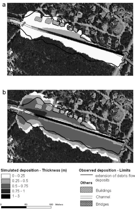
The Bingham and Coulomb-viscous rheologies were tested. As in the previous case, a calibration procedure was followed to determine the best set of parameters. Results for the shape of the deposits were good with both rheologies, al-though the Bingham rheology tended to under-predict the ex-tension of the deposit area (Fig. 5), and the Coulomb-viscous rheology tended to over-predict it. Most of the deposit area was predicted to be close to the first bridge, where the obsta-cle was located. From that point a debris flow body advanced downstream on the left bank, where the houses were located (Fig. 6). On the lower right bank there was some flooding directly from the torrent; the shape of the deposition in this area was well reproduced. There was more overflow from the channel on the right bank between the two bridges, co-inciding with the observed deposition. The thickness of the deposit was best predicted with the Coulomb-viscous rheol-ogy, as deposits more than 2 m thick were removed from the torrent banks near the bridge after the event finished. As in the previous case, the Bingham rheology resulted in a more homogenous and thin deposit. The best parameter sets were τC=400 Pa and µ=67 Pa s (Bingham) and τC=200, ϕ0=3.8◦
andµ=10 Pa s (Coulomb-viscous).
There are few reports of the modeling of canalized mud flows, but the Faucon 2003 event was modeled by Remaˆıtre (2006) using the BING code (Imran et al., 2001). The best parameter set for this simulation wasτC=404 Pa
andµ=122 Pa s, which are very close to the best Bingham rheology parameters in this study. The results of both sim-ulations are similar, although the final deposition maps of Remaˆıtre (2006) more accurately reproduced the deposi-tion shape around the bridge. Our model correctly repro-duced the observed deposition thickness, with most of the material remaining inside the channel, but in the results of Remaˆıtre (2006) the thickest deposition was concentrated around the houses on the left bank of the torrent. However, as these models were not run under equal initial and boundary conditions, comparison of the results is not definitive.
4 Discussion
Following a common approach for one-phase models, Mass-Mov2D assumes a homogeneous fluid with constant rheo-logical properties. Although this assumption may be appro-priate for mud flows, it is more critical in the case of debris flows where the separation of the solid and liquid phases is fundamental during the deposition phase. The inability to simulate the differing behaviors of the two phases is a limita-tion of one-phase models. Bingham-type flow models like the ones used in MassMov2D artificially simulate deposi-tion of the debris flow by introducdeposi-tion of a yield stress value. Other authors have proposed to change the flow regime dur-ing the simulation, followdur-ing pre-specified rules or rules im-posed as external conditions (e.g. McDougall et al., 2006).
Fig. 5. Simulation of the debris flow event of August 2003 in the
Faucon torrent, using Bingham (top) and Coulomb-viscous (bot-tom) rheologies. Simulation parameters were: τC=400 Pa and µ=67 Pa s; andτC=200 Pa,ϕ0=3.8◦andµ=10 Pa s, respectively.
Other alternative flow laws are rheological models based on the collisional dilatant model following the Bagnold theory (e.g. see Takahashi, 1991).
Fig. 6. Simulation of the debris flow event of August 2003 in the Faucon torrent, using Coulomb-viscous rheology. Spreading of the flow and
thickness at various times; 50 s (a), 100 s (b), 150 s (c), 200 s (d), 250 s (e), and 300 s (f). Simulation parameters were:τC=200 Pa,ϕ0=3.8◦
of granular flows (Pouliquen and Forterre, 2002; Mangeney et al., 2007). An alternative solution may be to include the coupling between the solid and the fluid fractions in or-der to model transient pore pressures, based on the grain-fluid mixture theory (Iverson, 1997; Iverson and Denlinger, 2001; Denlinger and Iverson, 2004). Such approaches, how-ever, have not yet generally been implemented in engineer-ing practice, and are beyond the original intentions of Mass-Mov2D.
The assumption of a fixed bed may also not be suitable for debris flows, for which erosion by scouring has been de-scribed as an important source of material. Sediment entrain-ment can also affect the properties of the debris flow, and thus greatly affect its behavior. A new version of MassMov2D, which will allow for a non-fixed bed, is currently under de-velopment.
5 Conclusions
MassMov2D is a numerical simulation model of the dy-namics (runout and deposition) of highly concentrated mass movements over complex topography. Due to the difficulties involved in obtaining direct information about the character-istics of debris and mud flows, numerical models are useful tools for hazard evaluation and mitigation, as they allow es-timation of relevant characteristics including the flow depth and the impact force.
The model proposed here is based on a depth-averaged form of the equations of motion for a fluid continuum, solved in a 2-D finite differences mesh. It can incorporate various constitutive relations for the flow resistance term, which al-lows the model to adapt to materials having different charac-teristics. The main drawback of the model is the assumption of a constant rheology. Further iterations of the model should address important issues, including the decrease in pore pres-sure during the simulation, allowing for a much more realis-tic simulation of debris flow behavior. However, this issue will remain a challenge for most one-phase codes.
In contrast with other codes for debris flow modeling, MassMov2D is implemented in a GIS environment. This fa-cilitates the tasks of preparing the input files and analyzing the model outputs, resulting in a user-friendly interface that facilitates use by non-experts in numerical computing. More-over, as the core equations of the model are implemented in an easy-to-learn scripting language, the model is especially suited to testing new modeling concepts.
The key inputs to the model can be created and manipu-lated using common GIS tools, making it is easy to develop simulation scenarios to fit real case studies. In this study we considered torrent debris flows in Wartschenbach (Aus-tria) and Faucon (France). Through a back-analysis pro-cess to establish the best set of parameters, the model was able to simulate the final spread and thickness of the debris flow deposits. These results provide evidence that the model
can accurately simulate real events, and justify its use as a tool in hazard analysis.
Acknowledgements. We thank D. Laigle, D. Rickenmann and J. H¨ubl for sharing the data on the Wartschenbach event. Data on the Faucon event was provided by A. Remaˆıtre, who also made valuable suggestions for creating the simulation scenario. We also thank A. Mangueney, M. Jaboyedoff and R. Genevois for their valuable comments on an early draft of the manuscript.
Edited by: T. Glade
Reviewed by: M. Jaboyedoff, R. Genevois, and another anonymous referee
References
Ancey, C.: Debris Flows and Related Phenomena, in: Geomorpho-logical Fluid Mechanics, edited by: Balmforth, N. J. and Proven-zale, A., Lecture Notes in Physics, 582, p. 528, 2001.
Arattano, M. and Franzi, L.: On the evaluation of debris flows dy-namics by means of mathematical models, Nat. Hazards Earth Syst. Sci., 3, 539–544, 2003,
http://www.nat-hazards-earth-syst-sci.net/3/539/2003/.
Bertolo, P. and Wieczorek, G. F.: Calibration of numerical models for small debris flows in Yosemite Valley, California, USA, Nat. Hazards Earth Syst. Sci., 5, 993–1001, 2005,
http://www.nat-hazards-earth-syst-sci.net/5/993/2005/.
Chen, H. and Lee, C. F.: Numerical simulation of debris flows, Can. Geotech. J., 37, 146–160, 2000.
Coussot, P., Laigle, D., Arattano, M., Deganutti, A., and Marchi, L.: Direct determination of rheological characteristics of debris flow, J. Hydraul. Eng., 124(8), 865–868, 1998.
Coussot, P.: Mudflow rheology and dynamics, Balkema, Rotter-dam, 1997.
Coussot, P.: Steady, laminar flow of concentrated mud suspensions in open channel, J. Hydraul. Res., 32(4), 535–559, 1994. De Blasio, F. V. and Elverhøi, A.: A model for frictional melt
pro-duction beneath large rock avalanches, J. Geophys. Res., 113, F02014, doi:10.1029/2007JF000867, 2008.
Denlinger, R. P. and Iverson, R. M.: Flow of variably fluidized gran-ular masses across three-dimensional terrain. 1. Numerical pre-dictions and experimental tests, J. Geophys. Res., 106, 553–566, 2001.
Denlinger, R. P. and Iverson, R. M.: Granular avalanches across ir-regular three-dimensional terrain: 1. Theory and computation, J. Geophys. Res., 109, F01014, doi:10.1029/2003JF000085, 2004. Fraccarollo, L. and Papa, M.: Numerical simulation of real
debris-flow events, Phys. Chem. Earth, 25, 757–763, 2000.
Greve, R. and Hutter, K.: Motion of a granular avalanche in a con-vex and concave curved chute: experiments and theoretical pre-dictions, Philos. T. R. Soc. A, 342, 573–600, 1993.
Han, G. and Wang, D.: Numerical modeling of Anhui debris flow, J. Hydraul. Eng., 122(5), 262–265, 1996.
Ho, A. and Li, E.: Proceedings of the 2007 International Forum on Landslide Disaster Management. Hong Kong Geotechnical Di-vision – Hong Kong Geotechnical Society – Geotechnical Engi-neering Office, Hong Kong, 2007.
¨
Osterreich, in: Proc. Internationales Symposium Interpraevent, Villach, Austria, 179–190, 2000.
Hungr, O. and McDougall, S.: Two numerical mod-els for landslide dynamic analysis, Comput Geosci, doi:10.1016/j.cageo.2007.12.003, in press, 2009.
Hungr, O., Evans, S. G., Bovis, M., and Hutchinson, J. N.: Review of the classification of landslides of the flow type, Environ. Eng. Geosci., VII, 221–238, 2001.
Hungr, O.: A model for the runout analysis of rapid flow slides, de-bris flows and avalanches, Can. Geotech. J., 32, 610–623, 1995. H¨urlimann, M., Rickenmann, D., and Graf, C.: Field and
monitor-ing data of debris-flow events in the Swiss Alps, Can. Geotech. J., 40(1), 161–175, 2003.
Hutter, K., Svendsen, B., and Rickenmann, D.: Debris flow model-ing: a review, Continuum Mech. Therm., 8, 1–35, 1996. Imran, J., Harff, P., and Parker, G.: A numerical model of submarine
debris-flow with graphical user interface, Comput. Geosci., 27, 717–729, 2001.
Iverson, R. M. and Denlinger, R. P.: Flow of variably fluidized gran-ular masses across three-dimensional terrain. 1. Coulomb mix-ture theory, J. Geophys. Res., 106, 537–552, 2001.
Iverson, R. M. and Denlinger, R. P.: The physics of debris flows – A conceptual assessment, in: Erosion and Sedimentation in the Pacific Rim (Proceedings of the Corvallis Symposium), IAHS Publ., 165, 155–165, 1987.
Iverson, R. M.: The physics of debris flows, Rev. Geophys., 35, 245–296, 1997.
Johnson, A. M. and Rodine, J. R.: Debris flows, in: Slope insta-bility, edited by: Brundsenn, D. and Prior, D.B., John Wiley, Chichester, 257–361, 1984.
Karssenberg, D., Burrough, P. A., Sluiter, R., and de Jong, K.: The PCRaster Software and Course Materials for Teaching Numer-ical Modelling in the Environmental Sciences, Transactions in GIS, 5(2), 99–110, 2001.
Laigle, D. and Coussot, P.: Numerical modelling of mudflows, J. Hydraul. Eng., 123(7), 617–623, 1997.
Laigle, D., Hector, A., H¨ubl, J., and Rickenmann, D.: Compar-ison of numerical simulation of muddy debris-flow spreading to records of real events, in: Proceedings of the Third Interna-tional Debris-Flow Hazards Mitigation: Mechanics, Prediction, and Assessment (DFHM) Conference, Davos, Switzerland, 635– 646, 2003.
Laigle, D.: A two-dimensional model for the study of debris-flow spreading on a torrent debris fan, in: Debris-flow hazards miti-gation: mechanics, prediction, and assessment, edited by: Chen, C.L., Proc. 1st International DFHM Conference, San Francisco (USA), 123–132, 1997.
Laigle, D.: Numerical modeling of mud/debris-flows and risk as-sessment on a torrent alluvial fan, in The Conference proceed-ings of the 28th IAHR congress held from 22–27 August 1999 in Graz, Austria, IAHR, Delft, 2000.
Major, J. J. and Iverson, R. M.: Debris-flow deposition: Effects of pore-fluid pressure and friction concentrated at flow margins, Geol. Soc. Am. Bull., 111, 1424–1434, 1999.
Malet., J.-P., Laigle., D., Remaˆıtre, A., and Maquaire, O.: Trigger-ing conditions and mobility of debris flows associated to complex earthflows, Geomorphology, 66(1–4), 215–235, 2005.
Mangeney, A., Bouchut, F., Thomas, N., Vilotte, J.-P., and Bristeau, M.-O.: Numerical modeling of selfchanneling granular flows and
of their levee/channel deposits, J. Geophys. Res., 112, F02017, doi:10.1029/2006JF000469, 2007.
Mangeney-Castelnau, A., Bouchut, F., Vilotte, J.-P., Lajeunesse, E., Aubertin, A., amd Pirulli, M.: On the use of Saint Venant equa-tions to simulate the spreading of a granular mass, J. Geophys. Res., 110(B9), B09103, doi:10.1029/2004JB003161, 2005. McDougall, S. and Hungr, O.: A model for the analysis of rapid
landslide motion across three-dimensional terrain, Can. Geotech. J., 41, 1084–1097, 2004.
McDougall, S., Boultbee, N., Hungr, O., Stead, D., and Schwab, J. W.: The Zymoetz River landslide, British Columbia, Canada: de-scription and dynamic analysis of a rock slide-debris flow, Land-slides, 3, 195–204, 2006.
Medina, V., H¨urlimann, M., and Bateman, A.: Application of FLATModel, a 2D finite volume code, to debris flows in the northeastern part of the Iberian Peninsula, Landslides, 5, 127– 142, 2008.
Naef, D., Rickenmann, D., Rutschmann, P., and McArdell, B. W: Comparison of flow resistance relations for debris flows using a one-dimensional finite element simulation model, Nat. Hazards Earth Syst. Sci., 6, 155–165, 2006,
http://www.nat-hazards-earth-syst-sci.net/6/155/2006/.
O’Brien, J. S. and Julien, P. Y.: Laboratory analysis of mudflow properties, J. Hydrol. Eng., 114, 877–887, 1988.
O’Brien, J. S., Julien, P. Y., and Fullerton, W. T.: Two-dimensional water flood and mudflow simulation, J. Hydraul. Eng., 119(2), 244–261, 1993.
Parsons, J. D., Whipple, K. H., and Simoni, A.: Experimental study of the grain-flow, fluid-mud transition in debris flows, J. Geol., 109, 427–447, 2001.
Pirulli, M., Bristeau, M. O., Mangeney, A., and Scavia, C.: The effect of earth pressure coefficient on the runout of granular ma-terial, Environ. Modell. Softw., 22(10), 1437–1454, 2007. Pouliquen, O. and Forterre, Y.: Friction law for dense granular
flows: Application to the motion of a mass down a rough inclined plane, J. Fluid Mech., 453, 133–151, 2002.
Press, W. H., Teukolsky, S. A., Vetterling, W. T., and Flannery, B. P.: Numerical recipes in C++, 2nd edn., Cambridge University Press, Cambridge, 2002.
Pudasaini, S. P., Wang, Y., and Hutter, K.: Modelling debris flows down general channels, Nat. Hazards Earth Syst. Sci., 5, 799– 819, 2005,
http://www.nat-hazards-earth-syst-sci.net/5/799/2005/.
Remaˆıtre, A., Malet, J.-P., Maquaire, O., Ancey, Ch., and Locat, J.: Flow behavior and runout modelling of a complex debris flow in a clay-shale basin, Earth Surf. Proc. Land., 30, 479–488, 2005. Remaˆtre, A., van Asch, Th. W. J., Malet, J.-P., and Maquaire, O.:
Influence of check dams on debris-flow run-out intensity, Nat. Hazards Earth Syst. Sci., 8, 1403–1416, 2008,
http://www.nat-hazards-earth-syst-sci.net/8/1403/2008/. Remaˆıtre, A.: Morphologie et dynamique des laves torrentielles:
Applications aux torrents des Terres Noires du bassin de Barcelonnette (Alpes du Sud), Ph.D. thesis, 2006.
Revellino, P., Hungr, O., Guadagno, F. M., and Evans, S. G.: Veloc-ity and runout simulation of destructive debris flows and debris avalanches in pyroclastic deposits, Campania Region, Italy, Env-iron. Geol., 45, 295–311, 2004.
Com-putat. Geosci., 10(2), 241–264, 2006.
Rodine, J. R. and Johnson, A. M.: The ability of debris, heaviliy freighted with coarse clastic materials, to flow on gentle slopes, Sedimentology, 23, 213–234, 1976.
Savage, S. B. and Hutter, K.: The Motion of a Finite Mass of Gran-ular Material Down a Rough Incline, J. Fluid Mech., 199, 177– 215, 1989.
Shieh, C. L., Jan, C. D., and Tsai, Y. F.: A numerical simulation of debris flow and its applications, Nat. Hazards, 13, 39–54, 1996. Takahashi, T.: Debris flow, IAHR-AIRH Monograph series,
Balkema, 1991.
Van Asch, Th. W. J., Malet, J.-P., van Beek, L. P. H., and Ami-trano, D.: Techniques, advances, problems and issues in numeri-cal modelling of landslide hazard, B. Soc. Geol. Fr., 178, 65–88, 2007.
Wang, C., Li, S., and Esaki, T.: GIS-based two-dimensional nu-merical simulation of rainfall-induced debris flow, Nat. Hazards Earth Syst. Sci., 8, 47–58, 2008,
http://www.nat-hazards-earth-syst-sci.net/8/47/2008/.
Wesseling, C. G., Karssenberg, D., Van Deursen, W., and Burrough, P. A.: Integrating dynamic environmental models in GIS: the de-velopment of a Dynamic Modelling language, Transactions in GIS, 1, 40–48, 1996.